Research Article | DOI: https://doi.org/10.31579/2637-8914/039
1 Institute of Health and Society, Faculty of Medicine, University of Oslo, Box 1130 Blindern, 0318 Oslo, Norway.
*Corresponding Author: Arne Torbjørn Høstmark, Institute of Health and Society, Faculty of Medicine, University of Oslo, Norway, Box 1130 Blindern, 0318 Oslo, Norway,
Citation: Arne Torbjørn Høstmark (2021) Studies to Explain Associations between Relative Amounts of Body Fatty Acids, 4(1); DOI:10.31579/2637-8914/039
Copyright: © 2021 Arne Torbjørn Høstmark, This is an open access article distributed under the Creative Commons Attribution License, which permits unrestricted use, distribution, and reproduction in any medium, provided the original work is properly cited.
Received: 27 January 2021 | Accepted: 05 February 2020 | Published: 01 March 2021
Keywords: correlation rules; relative amounts; distribution; biological regulation; fatty acids
Relative amounts of variables, such as body fatty acids, might be positively or negatively associated. The purpose of the present work was to investigate further, how such correlations might arise. One particular feature seemed to be that distributions of the variables were crucial for obtaining either positive or negative correlations, and for their strength, suggesting the name Distribution Dependent Correlations (DDC). The present work suggests that, with three positive scale variables, two of which (A, B) having very low variability relative to a third one (R), we should expect a positive association between percent A and percent B, the slope being estimated by the B/A ratio. Furthermore, we should expect a negative relationship between %R and %A (%B), in the current context. On the other hand, if A and B have high numbers and broad ranges relative to R, then %A should relate inversely to %B. Thus, ranges of A, B, and R seem to govern associations between their relative amounts, and alterations in the ranges have appreciable effects to change the associations. We suggest that evolution might utilize DDC to regulate metabolism, as suggested to occur with body fatty acids.
Fatty acids in blood and tissues are important in health and disease, and diet influences the body amounts [1-3]. Poly-unsaturated fatty acids with 20 or 22 carbon atoms serve as precursors for physiologically important regulatory molecules, concerning inflammatory and other diseases, i.e. the eicosanoids and docosanoids. Most organs and cell types produce these powerful metabolites, in reactions catasyzed by cyclooxygenases, lipoxygenases, and epoxygenases [4].
Eicosanoids derived from EPA (20:5 n3) may decrease inflammatory diseases [5, 6], improve coronary heart diseases [7, 8], and cancer [9]. However, a systematic Cochrane Review of selected studies questioned the beneficial effects of long-chain n3 fatty acids on all-cause and cardiovascular mortality [10].
When considering the beneficial health effects of foods rich in foods rich in n3 fatty acids, such as EPA [3, 7], we might anticipate many of the positive effects, if EPA works to counteract effects of AA (20:4 n6). This latter fatty acid is formed in the body from linoleic acid (LA, 18:2 n6), a major constituent in many plant oils, and is converted by cyclooxygenase and lipoxygenase into various eicosanoids, i.e. prostaglandins, prostacyclin, thromboxane, and leukotrienes [1,2]. AA derived thromboxane A2 (TXA2) and leukotriene B4 (LTB4) have strong proinflammatory and prothrombotic properties, and are involved in allergic reactions and bronchoconstriction [1, 2, 4]. Furthermore, AA- derived endocannabinoids may have a role in adiposity and inflammation [11]. Additionally, low serum EPA/AA ratio was a risk factor for cancer death in the general Japanese population [9].
Not only the eicosanoids, but also docosanoids, originating from C22 fatty acids (DPA, DHA), have strong metabolic effects. Among these latter compounds are protectins, resolvins, and maresins, which may strongly counteract immune- and inflammatory reactions [4]. Also eicosatrienoic acid, i.e. 20:3 n6 (dihomo-gammalinolenic acid, DGLA) may serve as precursor for eicosanoids [4]. However, to our knowledge, there are less data on eicosanoids derived from three other C20 fatty acids: the two eicosatrienoic acids 20:3 n3 and 20:3 n9 (Mead acid), and eicosadienoic acid (20:2 n6).
In order to achieve a balance between the metabolic influences of the many eicosanoids and docosanoids, we would expect a coordinated regulation of the precursor fatty acid percentages, e.g. of % EPA, %AA, %DGLA, and of other relevant fatty acid percentages. Indeed, we might expect in general that these particular percentages of the total sum of fatty acids were positively associated, so that an increase (decrease) in e.g. %AA would be accompanied by a concomitant increase (decrease) in other fatty acid precursor percentages as well, in order to obtain the required balance. We previously reported that that %AA, %EPA, and %DHA were positively associated in breast muscle lipids of chickens [12, 13, 14]. We also showed that this correlation outcome was related to the particular concentration distributions of the fatty acids, as suggested by similar outcomes with true values and surrogate random numbers, however sampled with the true ranges [13 - 17]. Computer experiments showed that altering ranges strongly influenced the correlation outcomes, suggesting the name Distribution Dependent Correlations, DDC [13, 17 - 22].
In addition, relative amounts of blood neutrophil granulocytes and lymphocytes seemed to be negatively associated because of their particular ranges [23].
In the present work, we raise the general question of whether relative amounts of particular variables are positively or negatively associated. Since DDC rules are general, we anticipate that they should apply to any unit system in nature. However, investigations specifically focusing upon this issue seem hard to find, in a literature search. The apparent lack of interest might possibly relate to a methodological concern encountered when correlating percentages of the same sum, since significant associations could arise mathematically [24]. On the other hand, it may not always be apparent whether positive (negative) associations between percentages of the same sum should be rejected as correlation bias, or rather be considered to have biological relevance. If DDC is an evolutionary regulatory principle, as previously suggested [19 - 21], we should expect strong correlations.
The aim of the present work was to examine in more detail, how percentages of the same sum might give strong correlations. First, we present theoretical considerations, and then show results of computer experiments to test the hypotheses.
Previously [20], we investigated the association between relative amount of arachidonic acid (20:4 n6) and percentage of e.g. eicosapentaenoic acid (EPA, 20:5 n3), in chicken lipids. From histograms, the physiological concentration distributions (g/kg wet weight) for the fatty acids were determined. Next the sum (S, g/kg wet weight) of all fatty acids was computed, as well as and the remaining sum (R) when omitting the couple of fatty acids under investigation, thereby apparently obtaining 3 positive scale variables. With these variables, and with surrogate random number variables, generated with the true concentration distributions, computer analyses as described in detail below, were carried out. For the purpose of the present work, the three positive scale variables were named A, B, and R. Previous analyses [19, 20] demonstrated that correlations between e.g. %A and %B depended upon the particular distribution (range) of each of the variables involved. Thus, we obtained similar correlation outcomes using the true (measured) values, or random numbers, if the ranges were like the measured ones.
A major part of the present work consists of computer experiments using random numbers to explore further, how distributions of A, B, and R might influence the association between relative amounts of the sum, S = A + B + R. Dependency between percentages is shown by the equation %A + %B + %R = 100. Using random numbers for A, B, and R, each of which sampled within defined ranges; we studied histograms, scatterplots, and correlations (Spearman’s rho). Computer experiments were performed, to study how alterations in the ranges of the random numbers might change associations between %A, %B, and %R. Several repeats were carried out, with new sets of random numbers (n = 200 each time); the general outcome was always the same, but corresponding correlation coefficients and scatterplots varied slightly.
We present the results mainly as scatterplots with correlation coefficients. In most of the computer experiments, the random numbers had uniform distribution, but we used random numbers with normal distribution as well, however obtaining qualitatively similar results. We used SPSS 27.0 for the analyses, and for making figures. The significance level was set at p < 0.05. We present further details under Results and Discussions.
We may encounter poor correlations in many contexts. However, if evolutionary selection is involved in associations between variables, we should probably expect correlations to be strong. In the reasoning below, and computer experiments, we try to find and explain conditions giving strong associations between percentages of the same sum. As outlined in the introduction, our previous observations with fatty acids initiated the current work.
Below, we extend the utilization of two main approaches to explain strong Distribution Dependent Correlations, i.e. 1) applying the equation of a straight line, and 2) considering the relationship between sum (S) of all variables and fractions (percentages) of S. Thus, the present study is an extension of our previous considerations and observations [13-17], to explain the correlation outcomes in more detail. For the purpose of the present work, it accordingly seems pertinent to include briefly some of the previous results.
Utilizing the Equation of a Straight Line (y = ax +b)
If S is the sum of many positive scale variables, S = A + B + C + …, we may simplify to S = A + B + R, i.e. %A + %B + %R = 100, or %B = -%A + (100 -%R), where R is the sum of all variables, except A and B. This equation seems to resemble the equation of a straight line, however involving percentage amounts of three unknown variables (A, B, R), each of which with a defined distribution (range). We previously considered in particular the equation, if 1) the expression (100 - %R) was approaching zero, and 2) if %R was approaching zero.
% R Approaching 100 [27]
The %A vs. %B Association
If %R consists of high values (close to 100) and (100 - %R) > %A, then the equation appears to approach %B = %A, apparently showing a linear positive association between %A and %B. The requirement (100 - %R) > %A is indeed satisfied, since the remaining value when calculating (100 - %R) would have to be divided between %A and %B. Hence, the slope of the %A vs. %B regression line should be positive. We may estimate the slope by utilizing maximum and minimum values of %B and %A, i.e. by the ratio (%Bmax - %Bmin)/(%Amax - %Amin). A more general equation would therefore be:

The subscript parentheses indicate ranges of %A and %B, and z = 100 - %R. Thus, z becomes increasingly small as %R increases.
The %R vs. %A (%B) Association
Since we have defined A and B to have very small values relative to R, it follows that also values of %A and %B should be small relative to %R. We rewrite the equation %A + %B + %R = 100, to be %B = -%R + (100 -%A). With very small %A - values, the equation would approach %B = -%R + 100, suggesting that %R and %B are inversely related. Similarly, the approximation %A = -%R + 100, suggest an inverse %R vs. %A association. Hence, in the current case, we should expect a negative %R vs. %A (%B) association.
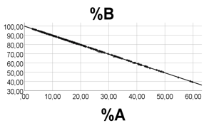
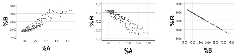
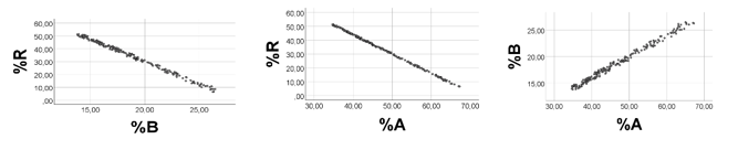
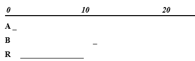
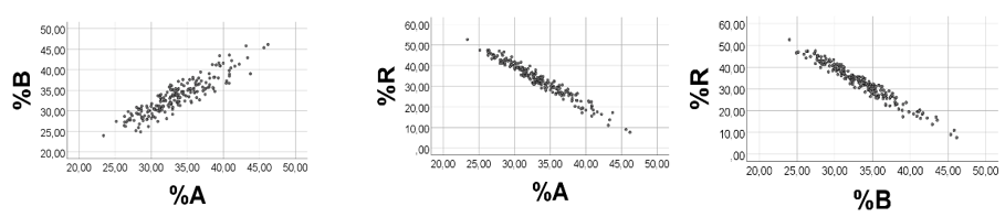
Computer testing: To obtain high %R values relative to %A and %B, we arbitrarily chose A 1.0 - 1.3; B 2.0 - 2.2; R 30 - 200. As shown in Figure 1, there was a strong positive association between %A and %B, and a strong negative relationship between %R and %A (%B). Spearman’s rho = 0.983 for %A vs. %B; rho = -0.992 (-0.998) for %R vs. %A (%B), p<0.001 for all, n = 200. Quartiles of %A, %B and %R were 0.8, 1.1, 1.6; 1.4, 1.9, 2.9; and 95.5, 97.1, 97.9, respectively. Thus, %R had high values relative to %A and %B. Skewness of %A, %B, and %R was 1.26, 1.24, and -1.24, respectively (SD 0.17 for all). Below, we explain this skewness outcome.

These results seem to be in line with the reasoning above: with very high %R values relative to %A and %B values, we should expect a positive association between %A and %B, and a negative relationship between %R and %A (%B). Additional computer experiments with a large number of varying ranges of the variables, however always keeping the above restrictions, showed results in keeping with the reasoning (results not shown).
% R Approaching Zero
If %R in the equation %B = -%A + (100 - %R) consists of very low values relative to %A (%B), we would expect a negative %A vs. %B association, since the equation in this case would approach %B = - %A + 100. However, in this case we should probably not expect that a decrease in %R would suffice to compensate a major increase in %A or %B. Hence, we should probably expect a poor correlation between %R and %A (%B).
Computer testing: To obtain very low values of %R relative to %A and %B, we arbitrarily chose A 10 - 50, B 20 - 67, R 0.10 - 0.13. Spearman’s rho = -1.000 for %A vs. %B, p<0.001, n =200; rho = 0.044 (-0.048), p = 0.532 (0.502) for %R vs. %A (%B). Quartiles of %A, %B and %R were 33.2, 40.8, 50.0; 49.9, 59.1, 66.6; 0.12, 0.15, and 0.18, respectively. Thus, values of %R were small relative to those of %A and %B.
Considering the Relationship between Sum (S) of the Variables and Their Fractions (Percentages) of S [25, 27]
Theoretical Considerations
We limit our reasoning to positive scale variables. Above we reasoned that, with a combination of two low-number variables (A, B) having narrow ranges relative to a third one (R), we might expect a positive association between %A and %B, and a negative relationship between %R and %A (%B). We now raise the question of whether also other than low numbers of A and B, however always with very low variability relative to R, might give positive %A vs. %B associations. Obviously, in this case the equation %B = -%A + (100 - %R) does not seem applicable, since (100 - %R) in many cases would not approach zero.
Two Positive Scale Variables (A and B) with Narrow Ranges Relative to a third One (R) with High Variability
We first consider the relationship between sum (S) of the variables and the A (B) fractions (percentages) of S. Intuitively; we would anticipate these fractions to decrease as S increases from lowest to highest value within the S - range. We should expect a positive correlation between A and B percentages, if both of them relate negatively to S. Furthermore, %R vs. %A (%B) should be inversely related, because %R should increase with increasing S. To explain this outcome in more detail, we omit ranges of the variables, and write A + B + R = S. The A, B, and R fractions of S are Af =A/S, Bf = B/S, and Rf = R/S, respectively.
Thus, Af = A/(A + B + R) = 1/(1 + B/A + R/A). However, since we - in the current context - define ranges of A and B to be very narrow, the B/A ratio is close to be a fixed number. Therefore, Af would approach Af = 1/(t +R/A) where t approaches a constant, i.e. t = 1 + B/A. Similarly, the B-fraction of S, Bf = B/ (A + B + R) = 1/ (1 + A/B + R/B), i.e. Bf = 1/ (k + R/B), where k is close to be a constant: k = (1 + A/B).
This means that R will largely govern the A (B) fractions. Thus, when R and S (being mainly composed of R) go from lowest to highest value, then Af = 1/(t + R/A), and also Bf = 1/(k + R/B), will go from the highest to the lowest value. Hence, S should relate inversely to the A- and B- fractions (percentages). This way of reasoning should apply to any positive values of A, B, and R, if ranges of A and B are very narrow relative to that of R. Accordingly, with this restriction, we should expect percent A to be positively associated with %B, wherever we place A, B, and R on the positive scale. However, increasing the A- and/or B-ranges (variabilities), and/or decreasing the R-range, would cause deviations from the above restrictions, and accordingly attenuate the %A vs. %B association, suggested to be reflected in scatterplots and correlation coefficients.
In brief, we may consider what happens to the B-fraction of S as the A-fraction increases. The A fraction of S, i.e. Af =1/(t +R/A), decreases when R goes from lowest to highest value. Simultaneously, also the B-fraction of S, i.e. Bf = 1/(k + R/B), decreases. Thus, the A and B fractions (percentages) of S should correlate positively, in the current context.
The R-fraction of S is Rf = R/S = R/ (A + B + R), i.e. Rf = 1/ (1 + z/R), where z is close to a constant, z =A + B. Therefore, the R fraction (and percentage) of S should increase with increasing R (from lowest to highest value), and accordingly also with increasing S, because R is the main contributor to S. Thus, S should be positively associated with %R, irrespective of where on the positive scale we place A, B, and R. It follows that %R should be negatively associated with %A and %B. In summary, from the relationships between S and A (B, R) percentages (fractions) of S, when putting the current restrictions on the ranges, we would anticipate a positive %A vs. %B association, and an inverse relationships between %R and %A (%B), wherever we encounter A, B, and R on the positive scale.
Two Positive Scale Variables (A and B) with Broad Ranges (High Variability) Relative to a Third One (R) with Low Numbers and Very Low Variability
To predict associations between percentages in this case, we use three ways of reasoning:
- Common sense: When approaching two variables only, their relative amounts should relate negatively.
- Utilizing the equation of a straight line [27]: If %A + %B + %R =100, the equation would approach %B = -%A + 100, if %R values are very small. Thus, %B should relate negatively to %A.
- Considering S vs. fractions of S [27]. Af = A/(A + B + R) = 1/[1 + (B +R)/A] should increase as B goes from highest to lowest value, and/or A goes from lowest to highest value. The B-fraction of S, Bf = B/(A + B + R) = 1/[1 + (A + R)/B] should increase as A runs from highest to lowest value, and B runs from lowest to highest value. Since Bf decreases as Af increases, we should expect a negative association between %A and %B, in the current case.
Thus, there seems to be two conditions giving strong negative correlations between fractions (percentages) of 3 positive scale variables. 1) If A and B have broad ranges and high numbers relative to R, then %A and %B should correlate negatively. 2) If A and B have very narrow ranges relative to R, then %R should relate negatively to %A and %B.
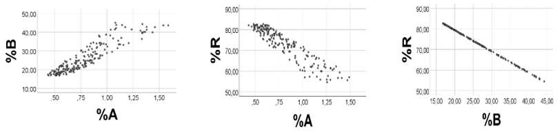
Computer Testing: To achieve high variabilities of %A and %B, and low %R values with low variability, we arbitrarily chose the following ranges: A 1 - 10; B 5 - 50; R 0.10 - 0.12. As shown in Figure 2, there was a strong negative association between %A and %B, rho = -1.000, p < 0.001, n = 200. Regression line for %A vs. %B: %B = - 1.010(0.001)*%A + 99.8(0.03). As anticipated, there was a moderate positive correlation between %A and A (rho = 0.671, p<0.001, n =200), and a negative association between %A and B (-rho = -0.658, p<0.001, n =200). Also correlations between %B and A (B) were as expected (not shown).
Chapter Summary and Some Additional Tests
In all of the previous cases, we aimed at selecting conditions suggested to give strong associations between relative amounts of three variables, and considered how each of the fractions would change within ranges of the variables.
Condition 1: Two variables (A, B) with very narrow ranges, and a third one (R) with broad range.
In this case, A and B are close to constants, and R is the only real variable. To assess possible correlations between their fractions (percentages), we need to consider what happens to each of them as R increases from lowest to highest value. Af = 1/[1 + (B +R)/A] should decrease as R increases, and so will also Bf =1/[1 + (A +R)/B] respond. Hence, %A and %B should correlate positively. In contrast, Rf = 1/[1 + (A +B)/R] should increase as R increases. Hence, %R should relate negatively to %A and %B.
Condition 2: Two variables (A, B) with broad ranges, and a third (R) with very narrow range
In this case, Af = 1/[1 + (B +R)/A] should increase as A increases and/or B decreases. Furthermore, Bf =1/[1 + (A +R)/B] should increase as A decreases and/or B increases.
Since Af increases as Bf decreases, we should expect %A and %B to relate negatively.
Additionally, Rf =1/[1 + (A +B)/R] should decrease as (A +B) increases. Since one particular value of (A + B) corresponds closely to one Rf value, we should expect a strong inverse association between Rf and (A + B). In contrast to this, there could be many combinations of A and B values giving the same sum of them (A + B). For example, if we choose A = 1, 2, or 3; and B = 7, 8, or 9, then the sum (A + B) could have these values: 8, 9, 10 (obtained with A =1); 9, 10, 11 (A = 2); 10, 11, 12 (A =3). Hence, we should probably not expect a strong correlation between Rf and A (B). A similar reasoning goes for associations between Rf and Af (Bf) as well. It is beyond the scope of this article to consider these associations in more detail.
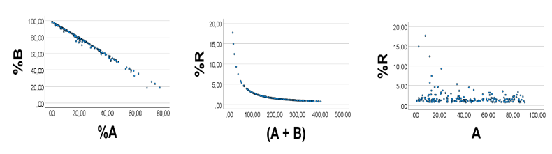
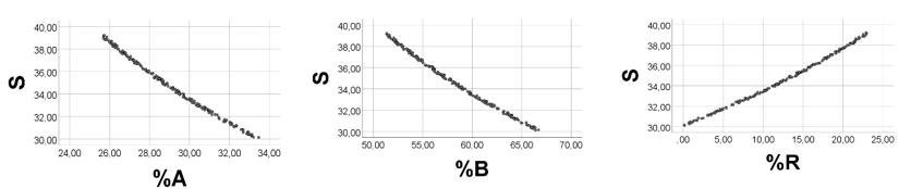
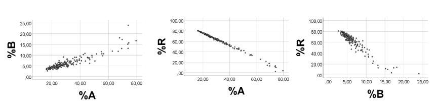
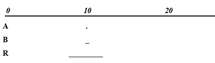
Computer test: To obtain broad ranges of A and B, and low numbers and narrow range of R, we arbitrarily chose: A 1 - 90; B 3 – 352; R 3.0 – 3.1, emphasizing that we chose these values just to illustrate a mathematical point, without any relationship to biology. In line with the above reasoning, %A was negatively associated with %B, rho = -0.995, p<0.001, n = 200, Figure 3, left panel. Correlations between %R and %A (%B) were poorer (scatterplots not shown): rho = 0.491 (-0.552), p<0.001, n =200. As shown in Figure 3 (middle panel), there was a strong curvilinear inverse relationship between %R and (A + B), and a poor association between %R and A (Figure 3, right panel), in keeping with the reasoning above.
Condition 3: Very narrow ranges of both A and R relative to B: In this case, we would have a situation with two near-constant variable (A and R) relative to the third variable (B). Above, we showed that this situation should give a positive association between %A and %R, and an inverse association between %B and %R(%A). Computer test: We made the following ranges: A 1-1.05; B 5 – 50; R 0.1 - 0.12. Correlations were as expected, %A vs. %R: rho = 0.992; %B vs. %R (%A): rho = -0.993 (-1.000); p< 0.001, n = 200 for all.
Condition 4: Very narrow ranges of both B and R relative to A: In this case, we would have two near-constant variables (B and R) relative to the third one (A). We should, accordingly, expect %R and %B to be positively associated, and %A to be negatively related to %R (%B). Computer test: We made the following ranges: A 1-10; B 5.00 – 5.05; R 0.10 - 0.12. Correlations were as expected, %B vs. %R: rho = 0.981; %A vs. %R (B): rho = -0.981 (-1.000); p< 0.001, n = 200 for all.
Condition 5: Narrow ranges of all of the variables (A, B, R): In this case, we would expect the degree of narrowing to govern the correlation outcome. For example, if A and B are more close to be fixed numbers than R, then we would anticipate %A and %B to be positively associated, and %R to relate negatively to %A (%B). Computer test: We chose A 1-1.002; B 5 – 5.002; R 0.1 - 0.2. The correlation outcome was as suggested, %B vs. %A: rho = 0.992 (Figure 4); %R vs. %A (%B): rho = -0.995 (-0.999); p< 0.001, n = 200 for all (not illustrated). Further computer experiments showed increasingly poorer %A vs. %B scatterplots (and correlation coefficients) in response to progressively narrowing the R-range (not shown), while keeping the ranges of A and B.

Slope of the Regression Line of the %A vs. %B Association, when A- and B- Ranges are Very Narrow Relative to the R Range
Approach #1 to Find the %A vs. %B Slope.
General consideration: Above, we utilized this equation %A + %B + %R =100, or %B = -%A + (100 -%R) to explain why %A correlates positively with %B, if %R values are very high. However, as demonstrated in the previous examples, we obtained positive %A vs. %B associations, and scatterplots close to straight lines, also with low numbers of R, and high numbers of A and B, on the condition that A and B had very narrow ranges relative to the R-range. We therefore need to consider in more detail the apparent linear positive %A vs. %B association. In this regard, we raise the question of what happens to %B (used as the ordinate = Y), as %A (the abscissa = X) increases, realizing that X as well as Y are functions of R. We use arbitrarily chosen values of X, within the X- range, emphasizing that we consider A and B as constants in the calculations below. If there is a linear relationship between X (= %A) and Y (=%B), then we should expect ΔY/ΔX to be constant.
First, we find the R (R1) that corresponds to particular values of X and Y. By definition, X = 100A/(A + B + R). We find R1, through the following steps: X (A + B + R1) = 100A; A·X + B·X +R1·X = 100A; R1 = (100A – A·X – B·X)/X. We next add one X-unit = ΔX.
Hence, X +1 = 100A/(A + B + R2); giving R2 = (100A - A - B - A·X - B·X)/(X+1).
To find ΔY, we use R1 and R2, and compute the corresponding Y-values. By definition, Y = 100B/(A+B+R); i.e.Y1= X·B/A. Similarly, Y2 =100B/(A+B+R2); i.e.Y2 = (X + 1)·B/A. Accordingly, ΔY = Y2 - Y1 = (X +1)·B/A – X·B/A = B/A, which is the change in Y corresponding to a one-unit increase in X, i.e. ΔY/ΔX = (B/A)/1= B/A.
Thus, in the current context, there should be a positive linear relationship between %B (“Y”) and %A (“X”), the slope being estimated by the B/A ratio. Below we show two examples to test this general reasoning. First, we consider a condition with two variables (A, B) having low numbers and very narrow ranges relative to a third variable (R) with broad range. Next, we use high numbers of A and B (with very narrow ranges) relative to R.
Computer Testing: With ranges: A 1.00 - 1.01; B 2.00 - 2.02; R 1.0 -10.0, A and B are close to constants. We found a perfect positive association between %A and %B (Figure 5); rho = 1.000, p<0.001, n = 200. Ranges of the relative amounts were 7.7- 24.7 (%A), 15.6 - 49.2 (%B), and 26.1 - 76.6 (%R). Skewness of %A, %B, and %R were 0.84, 0.84, and -0.84, respectively. Equation of the %A vs. %B regression line was: %B = 2.00 (0.00)*%A - 0.012 (0.024), i.e. a slope value equal to that found by the B/A ratio.
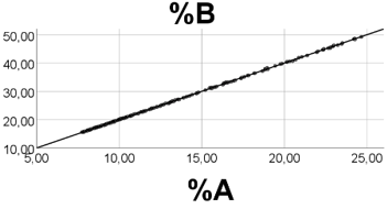
Thus, if both A and B have very low numbers and variabilities relative to R, then we find a positive and linear %A vs. %B association, the slope being well estimated by the B/A ratio.
With ranges A 50.00 - 50.05, B 20.00 - 20.02, and R 1 - 10.0, there was a perfect positive association between %A and %B (Figure 6), and a perfect inverse relationship (not illustrated) between %R and %A (%B); rho = -1.000 (-1.000), p<0.001 for all, n = 200.
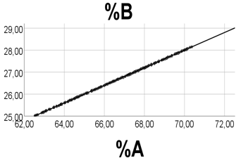
Ranges of relative amounts were 62.5 - 70.4 for %A, 25.0 – 28.2 for %B, and 1.5 -12.5 for %R, i.e. low values of %R relative to those of %A and %B. Equation of the %A vs. %B regression line was: %B = 0.40 (0.00)·%A - 0.018 (0.024), i.e. a slope value equal to that found by the B/A ratio. Accordingly, also if both A and B have very high numbers, but low ranges relative to R, then we find a positive and linear %A vs. %B association, the slope being well estimated by the B/A ratio.
Approach #2 to Find the %A vs. %B Slope.
General Consideration: The equation %B = -%A + (100 - %R) seems to resemble the equation of a straight line. The slope (ΔY/ΔX) of the regression line for the %A vs. %B association may be roughly estimated using maximum and minimum values of the A and B percentages, i.e. ΔY/ΔX = (%Bmax - %Bmin)/(%Amax - %Amin).
Hence, the equation %B = -%A + (100 - %R) could be written more precisely:
%B(p - q) = [(%Bmax - %Bmin)/(%Amax - %Amin)]*%A (r - s) + z
Subscript parentheses indicate ranges of %A and %B, and z = 100 - %R. The approximated slope value would accordingly be:
ΔY/ΔX = (100·Bmax /Smin – 100·Bmin/Smax)/(100·Amax /Smin – 100·Amin/Smax).
Since ranges of A and B are very narrow, we may do the following approximations:
Amax = Amin = A, and Bmax = Bmin= B. Thus, ΔY/ΔX = (B·Smax – B·Smin)/(A·Smax – A·Smin) = B/A. Thus, the slope may be estimated by the B/A ratio, and should approach +1 only if A approaches B. Conceivably, the slope value computed manually based upon the approximated values may deviate somewhat from the corresponding one found by the computer. This deviation should increase in response to increasing the A and/or B ranges.
Accordingly, if ranges of A and B are very narrow relative to that of R, the slope estimate of the %A vs. %B regression line should be little influenced by the magnitudes of the variables. Thus, with these restrictions laid upon A, B, and R variabilities, we suggest that the slope estimate of %A vs. %B (i.e. the B/A ratio) should apply to any R value on the positive scale, and to any sizes of the A and B numbers. Furthermore, with very narrow ranges of A(B), the scatterplot of the %A vs. %B association should be close to a line, since one particular value of %A (and of %B) corresponds closely to one S-value only. Hence, %A and %B should show a strong positive association. As explained above, the %A vs. %B scatterplot should improve (be poorer) in response to narrowing (broadening) the A and/or B ranges (variabilities), and also improve (be poorer) when increasing (decreasing) the R-range.
%R vs. %A (%B), when A (B) Ranges are Narrow Relative to R - Range
The equation %A + %B + %R =100 may be written %A = -%R + (100 - %B). If %B has very low values, this equation would approach %A = -%R + 100, showing a linear negative %A vs. %R association. The same reasoning goes for %B vs. %R, when %A values are small. Then, the equation would approach %B = -%R +100. Slope of the %R vs. %A regression line may be roughly estimated using maximum and minimum values of %R and %A, i.e. ΔY/ΔX = - (%Rmax - %Rmin )/(%Amax - %Amin). Similarly, slope of the %R vs. %B regression line may be estimated by ΔY/ΔX = - (%Rmax - %Rmin )/(%Bmax - %Bmin). In these cases, the previous simplification does not work, due to high R-variability.
Computer Experiments to Test in More Detail Associations between Percentages, and Applicability of B/A Ratio, if Ranges of A (B) are Narrow Relative to the R-Range
Initial tests of the %A vs. %B slope:
With A 0.100 - 0.102, B 0.200 - 0.201, and R 1- 2, we found that mean (SE) of the “computer- slope” was 1.99 (0.006), against min (max) 1.96 (2.01), n =200, when using the B/A ratio. If increasing the R- range to 1- 20, while keeping ranges of A and B, the mean “computer - slope” was 1.98 (0.001); with R 1 - 200, the slope was 1.99, and with R 1 - 2000, we found the slope value to be 1.98. We next made appreciable changes in the A, B and R sizes, i.e. A 1.00 - 1.02, B 50.0 - 50.05, R 1 - 10. The computer gave the following mean (SE) for the %A vs. %B slope: 49.2 (0.44); with the B/A –ratio, we found minimum (maximum) values 49.0 ( 50.1), n =200.We computer - tested slope values using many variations of A, B, and R ranges, however always keeping the A and B ranges very narrow. The slope values made by the computer were always close to that predicted by the B/A ratio (vide infra). As expected, the scatterplot became poorer in response to increasing the A and/or B range (or decreasing the R range), and the B/A ratio did not any longer seem a reliable estimate of the slope (scatterplots not shown).
Below we extend and systemize the computer experiments, to test how A-, B-, and R-percentages of S might correlate, in response to altering ranges of the variables. Additionally, we extend the testing of applicability of the B/A ratio to assess slope of the %A vs. %B association. In all of the experiments, we define ranges of A and B to be very narrow relative to the R-range.
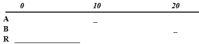
In most of the calculations, we use random numbers with uniform (rectangular) distribution. The correlation outcomes were, however, qualitatively the same with uniform and normal distribution of the random numbers, if corresponding ranges were equal. In each of the examples below, we illustrate schematically where we place A, B, and R on the scale; additionally, we show the exact ranges.
Example 1: Low numbers and ranges of A and B, relative to R

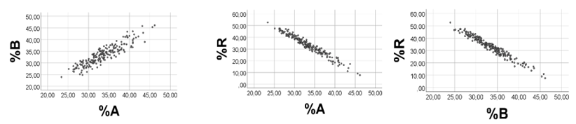
We arbitrarily chose the following ranges: A 0.10 - 0.15; B 4.0 - 4.2; R 5 - 20, and generated 200 uniformly distributed random numbers, based on these ranges. As shown in Figure 7, left panel, %A was positively associated with %B (Spearman’s rho = 0.913; %R was negatively associated with %A (%B): rho = -0.918 (- 1.000), p < 0.001 for all, Figure 7, middle and right panels. Slope (SD) of the %A vs. %B regression line, estimated by the computer, was 25.7 (0.78), against 26.7 - 42.0 using B/A ratio (min - max).
As anticipated, sum (S) of A + B + R correlated negatively with %A (%B) rho= -0.917 (-0.998), and positively with %R (rho = 0.998), p<0.001 for all, thereby explaining the positive %A vs. %B correlation, as well as the negative %R vs %A (%B) correlation.
Quartiles of the %A, %B, and %R distributions were 0.61, 0.73, 0.95; 19.6, 24.1, 31.1; and 67.9, 75.2, 79.8, respectively, i.e. showing low %A (%B) values relative to %R. Skewness of %A, %B, %R: 0.796, 0.778, and -0.776, respectively (SE 0.17 for all). Thus, A and B percentages had a moderate positive skewness, and %R a negative one.
Example 2: Numbers of A and B are higher than R, but A(B) ranges are much lower than the R range
We chose the following ranges: A 10.0 - 10.1; B 20.0 - 20.2; R 0 - 9, and generated 200 uniformly distributed random numbers based upon these ranges. As shown in Figure 9, left panel, %A correlated positively with %B (Spearman’s rho = 0.998, p<0.001). Furthermore, %R correlated negatively (Figure 9, middle and right panel) with %A (%B): rho = -0.999 (- 1.000), p < 0.001 for all. Slope (SD) made by the computer was 2.00 (0.01), and 1.98 - 2.02 (min – max) when using the B/A ratio.

As shown in Figure 10, sum (S) of the variables was negatively related to %A (%B); rho= -0.999 (-0.999), and positively associated with %R (rho = 1.000). These relationships may explain the positive %A vs. %B correlation, as well as the negative %R vs %A (%B) correlation. Quartiles of the %A, %B, and %C distributions were 27.2, 28.9, 30.8; 54.4, 57.8, 61.5; and 7.6; 13.4, 18.5, respectively, i.e. showing a quite different picture than that observed in Example 1. We found a modest positive skewness of %A, and %B (i.e. 0.367, and 0.381, respectively), and a modest negative one of %R (-0.376).
Example 3: The R- range includes ranges of A and B, both of which << R range

We chose the following ranges: A 10.0 - 10.5; B 4.0 - 4.2; R 1 - 15. As shown in Figure 11 (left panel), %A correlated positively with %B (Spearman’s rho = 0.993); %R was negatively associated with %A (%B): rho = -0.999 (- 0.996), p < 0.001 for all, n=200. Sum (S) of A, B, and R correlated negatively with %A (%B) rho= -0.996 (-0.997), and positively with %R (rho = 0.998), scatterplots not shown. These relationships to S may explain the positive %A vs. %B correlation, as well as the negative %R vs %A (%B) relationship.
The computer - made slope (SD) of the %A vs. %B regression line was 0.40 (0.003), and 0.38 - 0.42 (min and max) when using the B/A ratio. Quartiles of the %A, %B, and %C distributions were 39.9, 47.4, 55.4; 16.2, 19.0, 22.5; and 22.1, 33.5, 44.0, respectively, i.e. again showing a considerable difference from distributions found in Example 1 and 2. Skewness of %A, %B, and %R distributions were 0.561, 0.540, and -0.556, respectively (SE 0.17 for all). Thus, A and B percentages had a modest positive skewness, and %R a modest negative one (histograms not shown).
Example 4: Range of R is placed between A(B) ranges; range of A(B)<< R range
We chose A 0.10 - 0.12; B 11.0 - 11.2; R 1 - 10. Again, the positive %A vs. %B association prevailed (rho = 0.969), as well as the negative relationship between %R and %A(%B), rho = -0.970 (-1.000), p<0.001 for all; n= 200. S correlated negatively with %A (rho = - 0.969), and with %B (rho = - 0.999), and positively with %R (rho = 0.999), p<0.001, n =200; scatterplots not shown. Slope (SD) of the %A vs. %B regression line, made by the computer was 92.8 (2.3), and 91.7 - 112.0 (max and mean) when using the B/A ratio.
Example 5: Using A, B, and R with extremely low variabilities of all, however A(B) variability << R variability
We chose A 5.0000 – 5.0005; B 2.0000 – 2.0002; R 100.00 – 100.05. Again, the positive %A vs. %B association prevailed (rho = 0.961), as well as the negative relationship between %R and %A(%B), rho = -0.996 (-0.979), p<0.001 for all; n= 200. S correlated negatively with %A (rho = - 0.979), and with %B (rho = - 0.979), and positively with %R (rho = 0.986), p<0.001, n =200; scatterplots not shown. Slope (SD) of the %A vs. %B regression line, as made by the computer was 0.397 (0.008), and 0.400 when using the B/A ratio. Quartiles of the %A, %B, and % R distributions were 4.6715, 4.6721, 4.6725; 1.8686, 1.8688, 1.8690; and 93.4584, 93.4591, 93.4599, respectively. Thus, differences in quartiles appeared in the third decimal. Skewness of %A, %B, and %R distributions were -0.038, -0.033, and 0.037, respectively (SE 0.17 for all), i.e. all of the percentages had close to normal distributions (histograms not shown).
It might be questioned whether the above correlation outcome is related to using random numbers with uniform (rectangular) distribution. The outcome was, however, qualitatively similar also with normal distribution of the random numbers, as exemplified below.
Example 6. Using A, B, and R with normal distribution, and A(B)variability << R variability
We generated random numbers with normal distribution (n = 200), using the following mean (SD) values, i.e. A 1.0 (0.1); B 0.2 (0.02); R 2.4 (1.1). As shown in Figure 12, left panel, %A correlated positively with %B: rho = 0.879. The slope value was 0.196 made by the computer, and 0.200 by the B/A ratio. %R correlated negatively with %A (%B): rho = - 0.995 (-0.919); p<0.001 for all. S correlated negatively with %A (rho = -0.924), and with %B (rho = -0.922), and positively with %R (rho = 0.942), p<0.001, n =200; scatterplots not shown.
Quartiles of the %A, %B, and %R distributions were 23.6, 28.0, 35.3; 4.5, 5.7, 7.0; and 58.4, 66.5, 71.7, respectively, i.e. again showing a considerable difference from the distributions found in the previous examples. Skewness of %A, %B, and %R distributions were 2.49, 2.95, and -2.56, respectively (SE 0.17 for all). Thus, A and B percentages had a strong positive skewness, and %R a strong negative skewness (histograms not shown).
Example 7: Does a change in the R size influence the correlation between A, B, and R percentages of S, if using random numbers with normal distribution, and low variabilities of A and B?
In response to changing the R-values only, to be 8.0(2.4) instead of 2.4 (1.1), while keeping sizes and variabilities of A and B, i.e. A 1.0 (0.1); B 0.2 (0.02, the correlation outcome did not change much (%A vs. %B: rho = 0.853; %R vs %A: rho = -0.995; %R vs. %B: rho = -0.896); scatterplot not shown. Mean (SE) value of the “computer-made” slope of the %A vs. %B regression line was: 0.19 (0.01). We calculated ranges of A and B to be 0.76 -1.30, and 0.13 - 0.26, respectively. These ranges were broader than in the previous examples with uniform random numbers of A and B. Slope of the %A vs. %B regression line, as estimated with the B/A ratio (max and min), was 0.10 - 0.34, mean = 0.22. Quartiles of the %A, %B, and %R distributions were 9.0, 11.3, 13.7; 1.8, 2.1, 2.8; and 83.7, 86.5, 89.1, respectively, i.e. again showing a considerable difference from the distributions found in the examples above. Skewness of % A, %B, and %R distributions were 1.46, 1.95, and -1.53, respectively (SE 0.17 for all). Thus, A and B percentages had high positive skewness, and %R a high negative one.
Example 8: Normal distribution of A, B, and R; equal mean values (10.00) of all variables; however, variabilities (SD) of A and B are much lower than of that of R.
We chose mean (SD) values to be A 10.0 (0.3); B 10.0 (0.4); R 10.0 (4.0). Spearman’s rho for %A vs. %B: 0.930 (Figure 13, left panel); %R vs. %A(%B) rho - 0.982(- 0.980), Figure 13, middle and right panels; p<0.001 for all, n=200.
Sum of the variables (S) correlated negatively with %A (rho = - 0.978) and with %B (rho = -0.954), but positively with %R (rho = 0.983), p<0.001 for all; scatterplots not shown. This outcome is comparable to corresponding outcomes observed above when using uniformly distributed random numbers. Quartiles of the %A, %B, and %R distributions were 30.1, 33.4, 36.6; 30.0, 33.1, 36.2; and 27.5, 33.4, 40.0. Correlations: S vs. %A, %B, and %R; rho = -0.978, -0.954, and 0.983, respectively. Skewness of %A, %B, and %R were: 0.764, 0.850, -0.839 (SE = 0.172 for all). Thus, there was a moderate positive skewness of the %A and %B distributions, and a negative skewness of the %R histogram (not shown).
From the above considerations - and as supported by computer tests - it would appear that the particular ranges (variabilities) of A (B, R) govern the correlations between their relative amounts, as observed with uniform and normal distribution of random numbers. Additionally, we regularly observed that A and B percentages of S had positive skewness, and %R negative skewness. We previously commented on skewness [22], encountered with two variables having low variability (A and B) relative to a third one (R), as further examined below. Thus, the above reasoning and computer experiments seem to provide the following general rule: With three positive scale variables, two of which (A, B) having low variability relative to a third one (R), we should expect a positive %A vs. %B association, and a negative relationship between %R and %A (%B). This outcome seems to occur wherever we encounter the variables on the positive scale, and irrespective of using random numbers with uniform or normal distribution. Furthermore, slope of the %A vs. %B regression line may be well estimated by the B/A ratio.
Examples from Physiology: The B/A Ratio and Associations between Relative Amounts of Body Fatty Acids
In breast muscle lipids of chickens, we previously reported slope values of relative amounts of arachidonic acid (AA, 20:4 n6) vs. percentages of many other fatty acids, all of which having low variabilities relative to sum of the remaining fatty acids [20]. With reference to these observations, we should expect to find similarities between slope values of regression lines found by the computer, and those calculated manually, using the B/A ratio. We accordingly compared previously reported [20] slope values of seven associations, between %AA and percentages of other fatty acids. Numerators in the following fractions (in bold) are mean B/A-ratios, computed manually. Denominators are mean slope values of the regression lines, found by the computer. The results were: %AA vs. %20:5 n3, [1.7/1.2]; %AA vs. %20:2 n6, [6.2/5.6]; %AA vs. %22:5 n3,[1.0/0.8]; %AA vs. %20:3 n6, [3.9/3.2]; %AA vs. %18:0, [0.34/0.38]; %AA vs. %22:6 n3, [1.6/0.9]; %AA vs. %20:3 n3, [6.2/4.4]. These results seem to support that we, in the current context, may roughly estimate the slope by the B/A ratio. The outcome is in keeping with the reasoning above. We may add that all of the associations were generally strong ones, i.e. with rho > 0.7.
Alterations in Ranges and Correlations between Relative Amounts
With very narrow ranges of A and B relative to R, the A fraction of S will approach Af = 1/(t + R/A), and the B-fraction, Bf =1/(k + R/B), where t and k are close to be constants. In this case, one particular value of the A (B)-fractions (percentages) should correspond closely to one particular value of S, i.e. %A (%B) vs. S should be close to a line. This reasoning should apply to the positive S vs. %R relationship as well. However, when broadening the A and/or B ranges, the scatterplots should be poorer, since in this case, the above condition is disturbed. On the other hand, we would expect that narrowing the A and/or B ranges should improve the S vs. %A (%B) relationship. Additionally, any change in the R- range should influence %A and %B, since %A + %B + %R =100. Thus, increasing (decreasing) the values of R (%R) by broadening (narrowing) R towards higher (lower) values should decrease (increase) %A and %B, and accordingly improve (make poorer) the S vs. %A (%B) association, and therefore, also the %A vs. %B relationship.
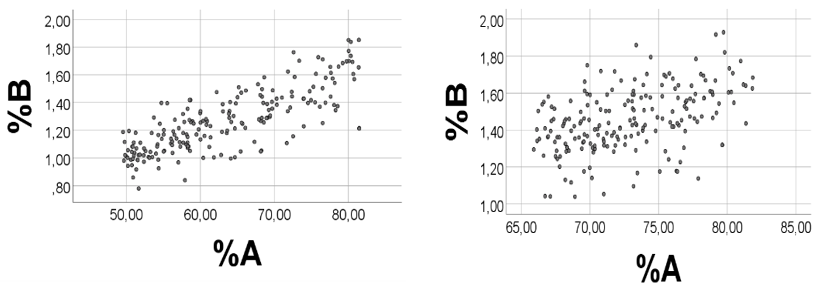
Below we show computer experiments to illustrate how alterations in ranges of A, B, and R may influence associations between the A and B percentages. We first re-examined the correlation outcome with ranges shown in Example 1, however using a new set of random numbers, i.e. ranges were A 0.10 - 0.15; B 4.0 - 4.2; and R 5 - 20. Spearman’s rho = 0.913 (p<0.001, n = 200) for %A vs. %B; rho = -0.918 (-1.000) for %R vs. %A (%B), Figure 14, left panel. According to the reasoning above, the association should improve (be poorer) if narrowing (broadening) the A and /or B ranges.
Changing ranges of A and B: We next narrowed the A range to be 0.10 - 0.11, and the B range to be 4.00 - 4.05 while keeping the R range. As expected, the scatterplot did improve (Figure 14, middle panel), rho = 0.993, p<0.001, n = 200. We then broadened the A range to 0.1 - 0.2, and the B range to 4.0 - 5.0, while keeping the R range. The %A vs. %B scatterplot was made poorer (Figure 14, right panel), rho = 0.728, p<0.001, n = 200. Additionally, the negative associations between %R and %A (%B) were changed according to suggestions (not shown).
Changing the R - range: We finally narrowed the R range to be 2 -10 instead of 0 -15, while keeping the A and B ranges, i.e. the chosen ranges were A 10.0 - 10.1; B 20.0 – 20.2; R 2 -10. The %A vs. %B scatterplot was made poorer (Figure 15, left panel), rho = 0.790 (p<0.001, n=200). When narrowing the R range further, to be 2-5, the scatterplot became even poorer (Figure 15, right panel), rho for %A vs %B 0.467, p<0.001, n = 200.
Conceivably, we might expect a positive %A vs. %B association, with slope estimate not far from the B/A ratio, also when conditions deviate somewhat from those mentioned (vide supra). Computer experiments confirmed this suggestion. These examples strongly support that variability of A, B, and R is the crucial factor governing associations between relative amounts of the variables.
Making Skewness
In many of the previous examples, we observed that distributions of A- and B- percentages of S had positive skewness, whereas %R had a negative skewness, raising the question of how to explain skewness of the relative amounts of A, B, and R.
We consider again S = A + B + R, where A and B have narrow ranges relative to the R-range. The A-percentage of S, %A = 100A/(A + B + R) = 100/(1 + B/A +R/A) = 100/( t + R/A), where t = 1+ B/A is close to a constant. Thus, R is the governor of %A, irrespective of where we place A and B on the positive scale. Furthermore, %A should relate inversely to R, since the denominator increases as R increases from lowest to highest value. Additionally, the decrease in %A per unit increase in R should be larger at low values of R than at high values, as for example illustrated using the following ranges: A 1.0 - 1.1, B 2.0 - 2.1, and R 1 - 100. Thus, with R = 1, %A = 100/(t + 1/A) = 100/( 1 +2/1 +1/1) = 25.0%. If increasing R one unit, %A = 100/(1+ 2/1 + 2/1) = 20%. However, a similar one-unit increase in R at the upper end of the R-range results in a much smaller decrease in %A, i.e. from 100/(1+ 2/1 + 99/1) = 0.98% to 100/(1+ 2/1 + 100/1) = 0.97%. Accordingly, the curvilinear negative association between %A and R should have the concave upwards, as also seen from the derivative of the approximated %A (%B) formula (not shown). Similar considerations should apply to the negative %B vs. R association.
The R-percentage of S is %R =100·R/(A + B + R) = 100/(1 + z/R) where z = (A + B) is close to a fixed number. Thus, %R should increase when increasing R from lowest to highest value. However, this effect should attenuate with increasing R-values, showing a positive curvilinear relationship between percent R and R, with the concave downwards. For example, when R goes from 1 to 2, then %R increases from approximately 100/(1 + 3/1) = 25% to 100/(1 + 3/2) = 40%. A similar one-unit increase in R at the upper end of the R-range, i.e. from R = 99 to R =100, is associated with a very small increase in %R, i.e. from 100/(1 + 3/99) = 97.05% to 100/(1 + 3/100) = 97.09%. This reasoning indicates that the concave should be downwards for to the positive relationship between %R and R. The finding that R is negatively associated with %A and %B explains that these percentages of S are positively associated. Furthermore, since %R is positively associated with R, percent R should be negatively related to %A and %B.
Furthermore, the relationships between R and %A, %B, and %R show that the number of cases associated with one unit decrease in %A (%B) is progressively falling as these percentages continue to decrease (Figure 16). The opposite happens for %R: the number of cases increases for each unit increase in %R. Thus, there will be a positively skewed histogram of %A (%B), and a negative one of %R (Figure 16, lower panels). Moreover, in the current example, R is the governor of skewness. Thus, an increase (decrease) in R range should increase (decrease) skewness of the histograms. However, from the mathematical formulas discussed above, and as illustrated in Figure 16 (top panels), we should not expect large differences in skewness of %A (%B, %R) in response to increasing the R-range above approximately R = 30, in this particular case. Similarly, if R is decreased below R = 30, then %A (%B) percentages should increase appreciably, and %R should decrease strongly. Computer experiments were in support of this reasoning (not shown). We emphasize that the R variability should be much higher than that of A (B), to achieve this outcome.
In the current example, skewness was high for relative amounts of the variables, i.e. 3.08, 3.08, and -3.08, for %A, %B, and %R, respectively (SE 0.17 for all; n = 200), as shown in Figure 16 , lower panels. As expected, %A correlated positively with %B (rho = 0.998), and %R negatively with %A (%B): rho = -0.999 (-1.000), p<0.001, n = 200.

Thus, provided that ranges of A and B are very narrow relative to that of R, the R-range will determine skewness of %A, %B, and %R, as well as correlations between the percentages, in the current case. Indeed, we may consider skewness as a mediator of the current correlations, as previously suggested [22].
The interplay between A, B, and R ranges concerning their influence upon skewness, and correlations is illustrated further by the next example, where we made a small increase in the A and B ranges, i.e. for A to be 1.0 - 1.5; for B 2.0 - 2.5; while keeping R 1- 2. This alteration had the effect that skewness was attenuated, to 0.16, 0.15, and 0.10 for %A, %B, and %R, respectively. With these ranges, %A and %B were not any longer significantly associated (rho = -0.012, p = 0.861). However, the inverse relationship between %R and %A (%B) prevailed modestly (%R vs. %A: rho = -0.586; %R vs. %B: rho = -0.785, p<0.001, n = 200).
Thus, we have explained how skewness of %A, %B, and %R are brought about, as well as their correlations, when S = A + B + R, and A (B) have very narrow ranges relative to R. In line with the a priori anticipations, we consistently observed a positive skewness of %A and %B histograms, and a negative skewness of the %R distribution. Furthermore, %A and %B did correlate positively, the slope being well estimated by the B/A ratio. As predicted, %R related negatively to %A and %B. Additionally, we showed that skewness and correlations might change appreciably in response to minor changes in the ranges of the variables.
Distribution Dependent Correlations and Associations between Body Fatty Acid Percentages
We recently reported that relative amounts of fatty acids that are precursors of eicosanoids (docosanoids) were positively associated in breast muscle lipids of chickens [13, 20, 21, 24]. Surprisingly at the time, the positive correlations could be well reproduced when random numbers were used in lieu of the true values of the fatty acids, provided that the random numbers were sampled with the true ranges [13, 14]. In this case, the concentration distributions of the various fatty acids were crucial for obtaining the correlations. For example, relative amount of arachidonic acid (AA, 20:4 n6) was shown to correlate positively with percentage eicosapentaenoic acid (EPA, 20:5 n3), and with some other eicosanoid precursor fatty acid percentages [20]. All of these fatty acids were low-number ones, with low variability, relative to sum of the remaining fatty acids. Since AA and EPA derived eicosanoids have opposing cellular effects [1-3], it was suggested that the positive association between %AA and %EPA might possibly serve to ensure a proper balance between the metabolic effects of these powerful metabolites. Furthermore, with percentages of oleic acid (OA, 18:1 c9) and AA, we observed a negative association [18]. Also in this case, we found significant inverse associations when using random numbers in lieu of the measured values of OA and AA, on the condition that their ranges had the true variabilities. Additionally, minor changes in ranges of the fatty acids had major effects on the mentioned correlation outcomes, suggesting that the correlations were distribution dependent ones.
Evolution and Distribution Dependent Correlations
We suggest that the principle of Distribution Dependent Correlations might be utilized in other contexts than with body fatty acids. Possibly, the suggested inverse relationship between relative amounts of lymphocytes and segmented neutrophil leukocytes could be another case of Distribution Dependent Correlations [24].
The present results indicate that variability is crucial for obtaining correlations (positive as well as negative) between percentages of the same sum. It is, however, beyond the scope of this article to discuss the many types of error in physiological research. In brief, genetics and external factors could influence variability, such as diet, physical activity, and environment in general. Additionally, errors related to time, sampling, storage, measurement, and information bias could influence spread of a variable. Conceivably, the between-subject variability should be greater than the within-subject one, due to between-subject variability of DNA per se, and differences in epigenetic influences, such as DNA methylation and histone modification. Accordingly, the many causes of variability do seem to be an argument in favor of considering Distribution Dependent Correlations (DDC) as a mathematical artifact, when it comes to possible physiological interpretations of such correlations. On the other hand, the mathematical principle of DDC could offer an excellent tool to regulate metabolism, raising the question of whether evolution might have utilized this principle. Our studies on body fatty acids [19 - 22, 25 - 27] seem in favor of this latter idea. Thus, by determining the within-person variability, i.e. where on the scale the variables are placed, it follows from the DDC rules described in this article, whether relative amounts will be positively or negatively associated, or not correlated at all. In other words, evolution could govern associations between percentages of the same sum, through regulating within-person distributions of variables. Since the mathematical rules giving Distribution Dependent Correlations are general ones, they might apply to any unit system in nature.
This work deals with theoretical considerations, and computer experiments, to explain associations between relative amounts of positive scale variables, as exemplified by body fatty acids. More studies are required to evaluate to what extent the suggested phenomenon of Distribution dependent correlations (DDC) is valid in the shown examples, and for other biological variables as well. Additionally, studies in various species should explore generalizability of the results. Furthermore, future studies should investigate the possible modifying influences upon DDC of environmental and lifestyle changes, including those related to diet and physical activity. Additionally, studies should clarify whether/how DDC relate to various disease conditions.
The present work explains why relative amounts of variables, such as body fatty acids, might be positively or negatively associated. One particular feature of such correlations seems to be that distributions (ranges) of the variables are crucial, suggesting the name Distribution Dependent Correlations (DDC). Thus, by directing variables to particular places on the scale, evolution might ensure that relative amounts of some variables must become positively associated, whereas percentages of others will correlate negatively. Since DDC rules are general, they should apply to any unit system in nature.
None
Variability: the width or spread of a distribution, measured e.g. by the range and standard deviation.
Distribution: graph showing the frequency distribution of a variable within a particular range. In this article, we also use distribution when referring to a particular range, a – b, on the scale.
Uniform distribution: every value within the range is equally likely. In this article, we may write, “Distribution was from a to b”, or “Distributions of A, B, and C were a - b, c - d, and e - f, respectively”.
OA = Oleic Acid (18:1 c9); LA = Linoleic Acid (18:2 n6); ALA = Alpha Linolenic Acid (18:3 n3); AA = Arachidonic Acid (20:4 n6); EPA = Eicosapentaenoic Acid (20:5 n3); DPA = Docosapentaenoic Acid (22:5 n3); DHA = Docosahexaenoic Acid (22:6 n3); DGLA= dihomo-gammalinolenic acid (20:3 n6)
“Low–number variables” have very low numbers relative to “high-number variables”.
Dear Editorial Team, Clinical Medical Reviews and Reports. My experience with the journal was highly positive. The peer-review process was rigorous, constructive, and completed in a timely manner. The reviewers provided valuable comments that helped improve the quality and clarity of our manuscript. The editorial office was professional, responsive, and supportive throughout all stages of the publication process. Communication was clear and efficient, and any questions were addressed promptly. Overall, I found the journal to maintain high scientific standards and an excellent publication workflow. I would be pleased to consider submitting future work to this journal. Best wishes from, Elena Popa.

It was my pleasure to submit my testimonial concerning the Reviewer Board of our Scientific Journal “Brain and Neurological Disorders”. The Reviewers focused on some modifications and their contribution was helpful. The ladies of our Editorial Office were also supported my efforts. It was my honor to have such a co-operation and I am looking forward for more collaboration.

Dear Grace Pierce, Editorial Coordinator of Journal of Clinical Research and Reports, Thank you for the speedy and efficient peer review process. I appreciate the fact that your peer reviewers do not take months to respond like with some other journals. I would also like to thank the editorial office for responding quickly to my questions. It is an excellent journal. I plan to submit more manuscripts in the future. Best wishes from, Robert W. McGee

Dear Grace Pierce, Editorial Coordinator of Journal of Clinical Research and Reports, Working with you and your team on our recent publication in JCRR has been a truly wonderful and enjoyable experience. The responses were prompt, and the reviewers were patient, constructive, and highly professional. One reviewer in particular gave me the feeling that a professor was carefully reading and commenting on my coursework, which was deeply touching. The entire process was straightforward and hassle‑free, with no tedious online forms to complete. I highly recommend this journal. Best wishes from, DR Aibing Rao, Head of R&D

I Appreciate the Opportunity to Share my Experience with the Journal of Clinical Research and Reports. The peer review process was timely and constructive, and the feedback provided helped improve the quality of our manuscript. The editorial office was professional, responsive, and supportive throughout the process, ensuring smooth communication and efficient handling of the submission. Overall, it was a positive experience collaborating with your team.

Dear Mercy Grace, Editorial Coordinator of Obstetrics Gynecology and Reproductive Sciences, We would like to express our gratitude for your help at all stages of publishing and editing the article. The editors of the magazine answer all the necessary questions and help at every stage. We will definitely continue to cooperate and publish other works in the Obstetrics Gynecology and Reproductive Sciences! Best wishes from, Alla Konstantinovna Politova,