Research Article | DOI: https://doi.org/10.31579/2637-8914/140
1 Professor & Head (Agricultural Economics), Agricultural College, Bapatla, Acharya NG Ranga Agricultural University (ANGRAU), Government of Andhra Pradesh, India
2 Postgraduate coordinator, Department of Agricultural and Food Economics, University for Development Studies (UDS), Ghana.
3 Professor (Agril. Economics), Department of Agricultural Economics, CARDS, Tamil Nadu Agricultural University (TNAU), Coimbatore- 641 003, Tamil Nadu, India.
*Corresponding Author: Adinan Bahahudeen Shafiwu, Postgraduate coordinator, Department of Agricultural and Food Economics, University for Development Studies (UDS), Ghana.
Citation: Ravi Kumar KN, Adinan B. Shafiwu and V. Saravanakumar (2023), Structure of Vegetables Demand in India during Covid-19 Regime: An Econometric Approach, J. Nutrition and Food Processing, 6(6); DOI:10.31579/2637-8914/140
Copyright: © 2023, Adinan Bahahudeen Shafiwu. This is an open access article distributed under the Creative Commons Attribution License, which permits unrestricted use, distribution, and reproduction in any medium, provided the original work is properly cited.
Received: 14 April 2023 | Accepted: 31 July 2023 | Published: 07 August 2023
Keywords: working-leser model; linear approximation almost ideal demand system; quadratic almost ideal demand system; southern india; vegetables demand
This study aimed to analyze the expenditure, own and cross-price elasticities of ten major vegetables in Southern India. using cross-sectional data from selected households in four southern states of India viz., Andhra Pradesh, Telangana, Karnataka and Tamil Nadu during 2020 to 2022. We use Working-Leser model, LA/AIDS model and QUAIDS model to compute elasticities and found QUAIDS model as the best fit. As expected the own-price elasticities for all the vegetables are negative and the expenditure elasticities are more than one, except tomato, lettuce and green sorrel. The cross-price elasticities showed that potato is complementarity to tomato, lettuce and green sorrel and the substitution effects of price change were not quite strong, except ivy gourd for bitter gourd; potato for ivy gourd and green sorrel for bitter gourd. Systematic differences in the absolute magnitudes of the expenditure elasticity and own-price elasticity were found and the demand for vegetables is largely influenced by the price change than the income/expenditure change. So, an appropriate price intervention policy by the Government may be more effective in influencing consumption pattern of vegetables enjoying more elastic demand.
India enjoys diverse agro-climatic conditions that is conducive to cultivate large number of vegetable crops and they facilitate the farmers towards adoption of farm diversification strategies. Being rich sources of vitamins and minerals, they further contribute to nutrition security of the population. In view of recent shift in consumption pattern in India from cereals to fruits, vegetables, meat and fish, the demand for vegetables is on the rise and other factors viz., increasing population, income, changing food habits, realizing nutritional value for boosting the immune in the context of COVID-19 pandemic also contributed for this. India holds 10.35 million hectares of land under vegetable cultivation (2019-20 National Horticulture Board 2nd advance estimates) with a productivity of 17.97 metric tonnes per hectare. It leads other countries in the world (next to China) in the production of vegetables accounting for 2.8 per cent of total cropped area and 13.38 per cent of total vegetable production. WHO has recommended a daily of intake at least 400 grams fruits and vegetables with an average serving size of 80 grams five times a day. However, their lower intake continued to prevail in different parts of the country due to different factors. The National Sample Survey Office (NSSO) highlighted that the average percapita consumption of fruits and vegetables in India is around 149-152 grams /day during this decade (2010-2020) and it is far below the recommended intake, but slightly better from the previous decade i.e., 120-140 grams/ day (https://www.ncbi.nlm.nih.gov). So, the vegetable consumption in India, on an average, is lower than WHO recommended levels. The recent COVID-19 pandemic has accentuated the both production and supply chain of vegetables in the country and this led to soaring prices of vegetables. Especially, the prices of vegetables like carrot, brinjal, bhendi, bitter gourd and cabbage have witnessed a hike, while the average prices of potato, tomato and leafy vegetables like green sorrel and lettuce have remained low compared to other vegetables.
Since, vegetables production and demand provide a promising economic opportunity for reducing rural poverty and unemployment in developing countries like India, the accurate estimates of price and income elasticities serve as important indicators for the formulation of market intervention scheme by the Government, trade, processing investments and other policies. However, despite their central importance, the robust estimates regarding demand elasticities are not available in the recent Indian context, especially with the prevalence of corona pandemic situation. It calls for estimating the consumers’ demand for vegetables in the context for setting R&D priorities and formulation of suitable production policy. Accordingly, ten major vegetables cultivated in Southern India are considered to estimate own-price, cross-price and expenditure elasticities of demand. The selected vegetables in this study are commonly available for the households across the selected States in Southern India. This will enable the researchers estimate the households’ budgetary allocations towards selected vegetables considering both substitution and complementarity issues.
The reviews discussed above and in the ensuing pages indicated that estimation of consumer demand for food has been highly researched among both theoreticians and empiricists in the past few decades. However, the present study differs from previous studies regarding the selection of only vegetable items that too during the COVID-19 pandemic period. This study will help the consumers in the allocation of budget towards purchasing vegetables keeping in view of their price and expenditure elasticities of demand and thus, safeguard them from escalating vegetable prices during COVID-19 regime. It also helps the farmers in the selection of crop (vegetable) enterprises in tune with the price elasticities. So, this study strikes a balance and win-win situation to both farmers and consumers towards improving the livelihood conditions of the former and to take care of demand preferences of the latter. Further, the earlier studies focused on aggregate food categories, such as ‘food’ or ‘meat’, or on specialized items such as beef, lamb, chicken, pork within meat etc. So, no studies were conducted earlier exclusively on vegetables that too in India in general and in Southern parts of India in particular between 2001 to 2020. As the nature of demand relationships for food will change over time as evidenced by several studies, the exclusive study on vegetables through employing cross-sectional data and that too in the context of COVID-19 pandemic deserve special mention. These relative merits will definitely enhance the contributions significantly different from those of earlier studies.
Study area and Data
The primary data are collected from 3000 households across four southern States in India (@ 750 households/State, Table 1). The data preparation for estimation of Working-Leser (W-L) model, Linear Approximation AIDS (LA/AIDS) and Quadratic AIDS (QUAIDS) models is the most important part, which comprises of several steps. First, the data on expenditure across different vegetables purchased are collected at weekly interval and by adding expenditure (four weeks) on all vegetables, we have total monthly expenditure of each household in one data file. In the second step, we selected 10 vegetables viz., potato, tomato, bhendi, carrot, brinjal, bitter gourd, lettuce, green sorrel, ivy gourd and cabbage across the selected States in view of their higher shares (compared to other vegetables) in monthly consumption expenditure of households and for which various forms of elasticities (Marshallian Uncompensated and Compensated (Hicksian)) were estimated. That is, we divided the monthly expenditure across 10 vegetables. In the third step, we computed monthly expenditure incurred on each selected vegetable for each household. Then, we computed expenditure share of each vegetable, as we have data on total expenditure incurred on ten vegetables and separate expenditure on each vegetable1. The expenditure share was worked out by dividing the food expenditure on each vegetable with total expenditure incurred on ten vegetables and these shares across all the vegetables will add up to 1. In the fourth step, we computed the price of each vegetable as it is the expenditure incurred on it divided by its quantity purchased. That is, the price of each vegetable is computed through dividing the monthly expenditure on it by quantity purchased by the consumer. The expenditure on vegetables are obtained for both regular and holiday periods. The data are collected for both purchased foods and self-supplied foods (home production). The analysis further assumed that the expenditure incurred on selected vegetables is separable from other food items and non-food items purchased, so as to estimate the demand for vegetables exclusively. The above requisite data are obtained from 3000 sample households in three different rounds of surveys in each district ie., during May, 2020 (1000 households), May 2021 (1000 households) and May 2022 (1000 households). That is the survey was repeated every year to obtain three observations per household over a span of three years. Combining the three rounds of survey data, a total of 2,860 observations are retained for this analysis. Primary data are collected from the sample households with the aid of pre-tested structured schedules (through personal interviews) regarding prices, quantities of major vegetables demanded and demographic characteristics of households (such as household head’s age, income, education (EDU), household size (HHS), location, sex etc).
1 - Note that, before computing shares, we replaced the missing values with zero for each food item.
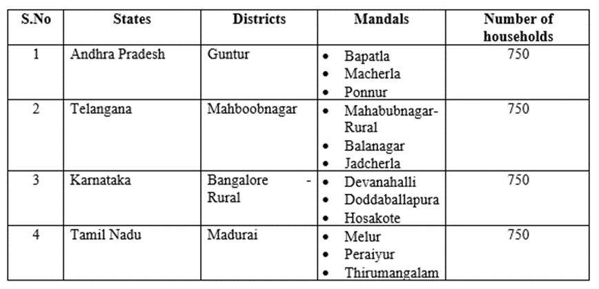
Table 1: Selection of households in three rounds of survey
In this study, we employed W-L model, LA/AIDS and QUAIDS models (Banks et al. 1997) to estimate expenditure share equations based on 10 major vegetables the households consume in four States in Southern India viz., Andhra Pradesh, Telangana, Karnataka and Tamil Nadu and to derive various elasticity parameters.
a. W-L model: This model was proposed by Working (1943) and Leser (1963) while, Intriligator et al. (1996) and Deaton and Muellbauer (1980a) elaborated the discussion on its operational form. In this model, the share of the food (vegetable) product is simply a direct function of the log of prices and total expenditure on all food items that are to be examined. The W-L food demand function can be expressed as:
 =
=  +
+  ln X +
  ln
ln +
+  ln m +
  (1)
(1)
where, i, j represents ten types of vegetables; wi = budget share of selected vegetables in the study, pj = price of ‘j’th vegetable; X = Total expenditure incurred on selected vegetables; m = demographic variables (education (EDU) & household size (HHS)), ε_i = random disturbances with zero mean and constant variance. So, the Equation 1 indicates that household food expenditure share may be calculated parametrically through the estimation of above functional equation which will relate the household food (vegetables) expenditure, prices of vegetables and demographic characteristics of the household. Expenditure elasticities of selected vegetables is given by (James, 2013):
 = 1 + (
 ) (2)
) (2)
where, e_i = expenditure elasticity and α_i1 = estimate of log of total expenditure on each of the selected vegetables.
Own and Cross (Marshallian/Uncompensated) price elasticities are given by:
 = -
= -  + (
+ ( ) (3)
) (3)
Where, i,j = 1…..n; δ_ij = Kronecker delta – in case of own price elasticity it will be equal to one while, in cross price elasticity it will be equal to zero; βij = coefficient of each selected vegetable.
Though W-L model has been used over the years in the consumption literature, the work of Deaton and Muellbauer (1980), has popularized the AIDS model, as the former one was collapsed for cross-sectional data.
b. LA/AIDS model: This study employed LA/AIDS because it can provide estimates of own price elasticity, cross price elasticity, and expenditure elasticity. Although AIDS is a non-linear model, the use of the Stone price index made it easier to estimate. Mathematically, the AIDS model used is as follows:
 =
=  +
+  ln
ln +
+  ln(
ln( ) + +
) + +  (4)
(4)
where, X is total household expenditure on the group of goods being analyzed, p_j is the price of the jth good, w_i is the budget share of the ith good (i.e., =
=  /X,
/X,  ,
,  , and
, and  are the parameters to be estimated, µ_i is the random disturbance term and the price index (p) is defined as:
ln p =  +
+  ln
ln +
+  ln
ln ln
ln (5)
(5)
To prevent non-linearity and reduce the effects of multicollinearity in the model, equation (5) is usually approximated by Stone’s Price Index: ln =
=  ln
ln (Stone, 1953). Further, household demand for vegetables not only depends on prices and income, but also on other socio-economic and demographic factors (m). The resulting LA/AIDS is given by:
 =
=  +
+  ln
ln +
+  ln(
ln( ) +
) +  ln m (6)
where, x (= X/m) is the per capita household expenditure and x (= X/m) is the effect of demographic variable on budget share in addition to the effect of per capita real household expenditure ( ).
).
From the estimated parameters above, the demand elasticities are calculated. The expenditure elasticity (η_i), which measures sensitivity of demand in response to changes in consumption expenditure, is expressed as:
 = 1 +
= 1 +  (7)
(7)
The uncompensated own price elasticity ( ) and cross price elasticity (
 ) measures how a change in the price of product ‘i’ and of other product ‘j’ affects the demand of product ‘i’ respectively, keeping total expenditure constant. The uncompensated own and cross price elasticities are worked out as follows:
 = - 1 +
  -
-  (8)
(8)
 =
=  -
- 
 (9)
(9)
The compensated price elasticities (own and cross ie.,  and
and  respectively), which measures the price effect on the demand assuming the real expenditure X/
 constant, is described as:
 = - 1 +
  +
+  (10)
(10)
 =
=  +
+  (11)
(11)
c. QUAIDS model: Assume a consumer demand for a set of ‘k’ vegetables with a budget outlay of ‘y’ from the household’s income, ‘m’. According to Poi (2002), the household’s expenditure share for vegetable ‘i’ is given as:
 =
= 
where, p_i is the price paid for good ‘i’, q_i is the quantity of good ‘i’ purchased. From the definition of ‘y’,
 = 1
= 1
The QUAIDS model assumes that household preferences belong to the following quadratic logarithmic family of expenditure functions.
ln(u,p) = ln a(p) +  (12)
(12)
where, ‘u’ is utility, ‘p’ is a vector of prices, ‘a(p)’ is a function that is homogeneous of degree one in prices, ‘b(p)’ and ‘λ(p)’ are functions that are homogeneous of degree zero in prices.
The quadratic AIDS model of Banks, Blundell, and Lewbel (1997) depend on the indirect utility function.
ln V(p,y) =  (13)
(13)
where ‘y’ is total expenditure on vegetables. The specific functional form is
λ(p) = 
 = 0
= 0
where, i = 1…..,k stand for the number of vegetables entering the demand model and ‘ln a(p)’ is the transcendental logarithm function:
ln a(p) =  +
+  +
+ 
 (14)
(14)
 is the price of good ‘i’ for i = 1 ……. k, b(p) is the Cobb Douglas price aggregator
b(p) = 
and
λ(p) = 
The fact that  = 1 refer to as the adding up condition and this condition is satisfied, if
 = 1
= 1  = 0
= 0  = 0 and
  = 0
= 0 
The adding up restrictions are not testable, and are imposed by dropping one of the share equations and estimating the remaining equations.
Moreover, since demand functions are homogeneous of degree zero in (p,y),
 = 0
= 0 
Slutsky symmetry implies that
 =
= 
Usually, it is difficult to estimate α_0 directly. The share equation for QUAIDS model can be obtained by applying Roy’s identity:
 =
=  +
+  +
+  ln{
ln{ }+
}+ (15)
(15)
where,  and
and  represent vectors of prices of ith and jth commodities, and
a. Socio-economic and demographic characteristics
Regarding descriptive statistics (mean, Standard Deviation (SD), minimum and maximum values, Table 2), in terms of budget allocation per month, leafy vegetables viz., green sorrel enjoyed the highest share (23.39%) followed by lettuce (16.24%). These two are followed by tomato (12.12%), bitter gourd (12.01%), bhendi (11.26%) and potato (7.13%), while carrot (4.14%) had lowest budget share. With respect to prices of selected vegetables, again leafy vegetables viz., green sorrel and lettuce are offered at lower prices viz., Rs.12.57/kg and Rs. 12.69/kg. The above two leafy vegetables are consumed across divergent socio-economic strata of the selected sample. It is surprising that during COVID-19 regime, the expenditure shares are higher on these two vegetables compared to other vegetables in view of declined income earning opportunities. So, nearly every household consume these two leafy vegetables and total expenditure on them forms a significant proportion (40%) of households’ monthly vegetables budget. The low monthly expenditure share on carrot (4.14%) is not also unexpected because of its highest price in the market and hence, it lacks general acceptability due to fluctuating monthly incomes of majority of the consumers during COVID-19 regime. The findings further revealed that prices of lettuce and green sorrel had lower SD, while the carrot price has the largest SD. The mean and SD for the total vegetables monthly expenditure are Rs. 2110.76 and 223. The mean values for age, EDU and HHS are 45.86, 10.14 and 5.21 respectively. The number of males who are heads of household are more (2156) compared to female-headed households (844) in the selected sample. Majority of the households belong to urban area (56%) and remaining 44 per cent reside in rural area. Figure 1 shows the scatter plot of expenditure on vegetables (EXP) against age and HHS. This shows that there is positive association between EXP, HHS and age.

| Variables & Units | n | Frequency | Mean | SD | Min | Max |
| Age (years) | 2860 | 45.86 | 10.88 | 28.00 | 65.00 | |
| EDU (years) | 2860 | 10.14 | 5.84 | 0.00 | 20.00 | |
| HHS (Number) | 2860 | 5.21 | 2.29 | 2.00 | 9.00 | |
| Location | ||||||
| Rural (Number) | 1317 | |||||
| Urban (Number) | 1683 | |||||
| Monthly income (Rs) | 2860 | 20721 | 8106 | 7005 | 34979 | |
| Sex | ||||||
| Male (Number) | 2156 | |||||
| Female (Number) | 844 | |||||
| Potato price (Rs/kg) | 2860 | 47.63 | 8.45 | 30.00 | 60.00 | |
| Tomato price (Rs/kg) | 2860 | 14.91 | 6.96 | 5.00 | 25.00 | |
| Bhendi price (Rs/kg) | 2860 | 67.58 | 8.65 | 55.00 | 80.00 | |
| Carrot price (Rs/kg) | 2860 | 97.91 | 24.26 | 75.00 | 120.00 | |
| Brinjal price (Rs/kg) | 2860 | 59.61 | 9.90 | 45.00 | 75.00 | |
| Bitter gourd price (Rs/kg) | 2860 | 89.69 | 7.11 | 80.00 | 100.00 | |
| Lettuce price (Rs/kg) | 2860 | 12.69 | 2.49 | 10.00 | 15.00 | |
| Green Sorrel price (Rs/kg) | 2860 | 12.57 | 2.66 | 5.00 | 20.00 | |
| Ivy gourd (Rs/kg) | 2860 | 29.11 | 3.19 | 11.25 | 26.18 | |
| Cabbage (Rs/kg) | 2860 | 18.84 | 6.24 | 10.27 | 29.21 | |
| w1 (%) - Potato | 2860 | 7.13 | 0.10 | 0.06 | 0.55 | |
| w2 (%) - Tomato | 2860 | 12.12 | 0.02 | 0.00 | 0.11 | |
| w3 (%) - Bhendi | 2860 | 11.26 | 0.10 | 0.04 | 0.55 | |
| w4 (%) - Carrot | 2860 | 4.14 | 0.07 | 0.06 | 0.42 | |
| w5 (%) - Brinjal | 2860 | 4.31 | 0.07 | 0.03 | 0.39 | |
| w6 (%) - Bitter gourd | 2860 | 12.01 | 0.05 | 0.05 | 0.32 | |
| w7 (%) - Lettuce | 2860 | 16.24 | 0.01 | 0.01 | 0.08 | |
| w8 (%) - Green Sorrel | 2860 | 23.39 | 0.03 | 0.00 | 0.14 | |
| w9 (%) - Ivy gourd | 2860 | 5.21 | 0.03 | 0.00 | 0.11 | |
| w10 (%) - Cabbage | 2860 | 4.19 | 0.02 | 0.00 | 0.09 | |
| Monthly expenditure on vegetables (EXP) (Rs) | 2860 | 2110.76 | 223.00 | 165.00 | 3240.00 | |
| lnexp | 2860 | 7.65 | 0.21 | 6.76 | 8.08 | |
Table 2: Descriptive Statistics for selected variables
b. Estimated results of W-L Model: Table 3 shows expenditure elasticities (indicate the percentage change in the amount spent on a vegetable as a result of the percentage change in income of the household, Khanal et al., 2017) of selected vegetables are positive implying that they are all normal goods. That is, the demand for these goods increase with increase in income of the household. Among the selected vegetables, tomato (0.6227) was found expenditure inelastic which shows that rise in the total expenditure by one per cent would tend to cause an increase in its expenditures only by 0.62 percent. This result is in tune with the Kenyan study results of (Ahmad et al, 2015), who classified chicken as the necessity due to its rearing and readily availability for consumption. A close examination of the findings also indicate that lettuce and green sorrel were near unitary expenditure elastic. These results are in tune with the findings of Talijaard et al., 2004 study on the consumer demand for pork. However, for other vegetables like potato, bhendi, carrot, brinjal, bitter gourd, ivy gourd and cabbage the elasticity coefficients are greater than one (luxury goods). Carrot (1.8107) and bitter gourd (1.5526) expenditures are most elastic, which means when the household’s expenditures will increase by one per cent, their consumption will increase by 1.81 and 1.52 percents respectively. This finding is in line with the Talijaard et al., 2004, who observed that mutton and beef expenditure elasticities greater than one in the diet of African households. These findings also infer that tomato, lettuce and green sorrel being expenditure inelastic, these are largely consumed especially by the consumers with fluctuating income levels. On the contrary, other vegetables such as carrot and bitter gourd and other luxury goods being more expenditure elastic, they are less consumed by the consumers.

Table 3: Estimated results of the W-L Model
The own price elasticities of selected vegetables are negative in accordance with the law of demand. Further, they are less than one, except for bitter gourd (-1.0321), lettuce (-1.4135), green sorrel (-1.3998) and ivy gourd (-1.0052) indicating that their demand is highly price elastic ie., their quantities demanded are highly sensitive to their respective price changes (Table 3). These results are in line with the findings of Dhraief et al., 2013 indicating that for a commodity with high elastic demand, an increase in the price would drop the quantity demanded sharply and vice versa. It is interesting that leafy vegetables (lettuce (-1.4135) & green sorrel (-1.3998)) has highest own price elasticity and lowest expenditure elasticity (lettuce (0.9892) & green sorrel (0.9616)) indicating that their demand is more driven by changes in their prices rather than the income/expenditure change of the household.
Regarding cross-price elasticity of demand, as number of substitutes of a commodity decreases, elasticity or price sensitivity decreases. The findings revealed that for example, potato is complementary to tomato (-0.6078), carrot (-0.7154) and green sorrel (-0.6193) implying that they are gross complements for potato, while other vegetables are gross substitutes for potato. The quantity consumption of ivy gourd enjoy the strongest substitution response for the price of bhendi (0.9198) and the substitution holds good even in the reverse direction (0.7025). The next substitution response is the consumption of potato for the price of cabbage (0.7583), followed by green sorrel for carrot (0.7426). The strongest complementarity relationship is between consumption of green sorrel and potato (-0.7309) followed by potato to carrot (-0.7154) implying that the selected households consume curries with combinations from potato and green sorrel or potato and carrot.
c. Estimated results of LA/AIDS and QUAIDS models: Table 4 shows the results of the estimated parameters of the LA/AIDS model with demographic variables (EDU & HHS). The reported estimates and their respective Standard Errors (SEs) indicated that all of the 55 price effects (γ_ii) are significant either at 1 and 5 per cent significance levels indicating that there is much quantity response to the movement in relative prices. So, a change in price of a vegetable leads to a systemic change in the expenditure share of that vegetable in the total consumption expenditure. The coefficients of the EDU and HHS are positively related to the expenditure shares across the selected vegetables. This result is in line with Horowitz (2002) and Olorunfemi (2013).
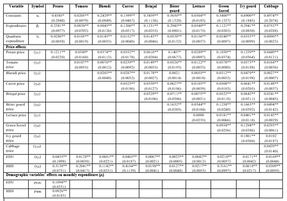
The estimation results of QUAIDS model (Table 5) revealed similar findings with respect to price effects as in LA/AIDS model ie., all parameters are statistically and significantly different from zero, except in few isolated cases. This finding is in contrast with the study conducted by Surabhi (2008), as the squared terms of expenditure are significant only for two of the selected food items considered in his study. The alpha coefficients (intercepts) are statistically significant and positive for all the selected vegetables. For the parameters of both linear and quadratic expenditures, all are statistically significant and the quadratic expenditure values are consistently smaller in magnitudes than the linear expenditure estimates, as would be expected. The statistical significance of both linear and quadratic expenditure terms indicate that the total vegetables budget is an important determinant for the expenditure shares among the selected vegetables and their consumption is very sensitive to expenditures incurred. Regarding the demographic variables, both EDU and HHS had positive and statistically significant influences on the demand for all the selected vegetables. However, the estimated values reported for HHS are stronger operationally compared to the effects of EDU (quite close to zero). These results are quite expected, since demand for various vegetables would depend more on the HHS (relative to EDU) besides the conventional price and quantity factors. These findings on the influences of demographic factors on vegetables expenditure is in line with the results from most demand studies (Christensen, 2014; Dong et al, 2004; Gould, 2002; Gould and Villarreal, 2006; Gould et al, 1991; Hovhannisyan and Gould, 2011). So, at any given level of prices and expenditure, as HHS increases, members of the household are forced to adjust their patterns of demand towards cheap food items such as lettuce, green sorrel and tomato among others, and away from expensive vegetables like carrot, bitter gourd, bhendi and brinjal.
Among these two models, the interpretation of the results from QUAIDS model is more valid, as the Wald test (χ2= 276.52, Prob≥ χ2=0.0000) is highly significant indicating that the lambda coefficients are jointly significantly different from zero thereby, the quadratic expenditure terms are important. This shows the superiority of QUAIDS model over the LA/AIDS model. This finding is in line with that of Luca (2007), Olorunfemi (2013), Isaac et al (2020) etc. Hence, in the future pages, the interpretations for both price and expenditure elasticities are discussed in terms of QUAIDS model.

Note: ** & * - Significant at 1 and 5 per cent levels respectively
Table 4: Estimated results of the LA/AIDS Model
Note: ** & * - Significant at 1 and 5 per cent levels respectively
Table 5: Estimated results of the QUAIDS Model
d. Marshallian (uncompensated) own and cross-price elasticities: Marshallian (uncompensated) price elasticity describes the percentage change in the quantity demanded of a vegetable as a result of its price change and it is greater than Hicksian (compensated) price elasticity because, the former contains both income and substitution effects (whereas, the Hicksian price elasticity contains only the substitution effect). Table 6 presents the Marshallian (Uncompensated) own and cross-price elasticities calculated at their sample means. The uncompensated own-price elasticities (diagonal elements in QUAIDS model) are with expected negative signs in consistent with the theory and found statistically significant at 5 per cent level. They describe, how demand for a vegetable changes when price changes, holding money income constant (Issac et al, 2020). It is interesting that the estimates for the own-price uncompensated elasticities are smaller in magnitude compared to compensated own-price elasticity estimates for all the selected vegetables (Tables 6 and 7). It was also found that the quantities demanded of all the selected vegetables are highly sensitive to price changes, as the estimated own-price elasticities are almost close to or slightly above -1.00. This is because of declined income opportunities among majority of the households both in rural and urban areas during COVID-19 regime. This made them to be highly cautious in spending their limited income on highly priced vegetables in the open market. So, when the prices of the vegetables increase, the quantities demanded by the household decreases significantly. Though vegetables usually represent the necessary goods, these results are found surprising during COVID-19 pandemic. The results further showed that own-price elasticities for majority of the vegetables are significantly less than zero exhibiting inelastic relationship with only few (bitter gourd, lettuce, green sorrel and ivy gourd) being elastic. Bhendi enjoyed more inelastic demand (-0.8477) among the selected vegetables in view of its benefits for heart health, blood sugar control, anti-cancer properties etc. Hence, the consumers allocated 11 per cent of total vegetables outlay on this commodity to check post-COVID health issues. The findings also showed that ivy gourd enjoy the highest Marshallian price elasticity (-1.6616), followed by green sorrel (-1.4795), bitter gourd (-1.2962), lettuce (-1.0410), and tomato (-0.9697). So, ivy gourd is most responsive to price change compared to other vegetables. That is, an increase in price of ivy gourd by one per cent, it causes a decrease in its demand by 1.66 per cent (Anindita, 2020).
| LA/AIDS Model | ||||||||||
| Potato | Tomato | Bhendi | Carrot | Brinjal | Bitter gourd | Lettuce | Green Sorrel | Ivy gourd | Cabbage | |
| Potato | -0.9595 | -0.0168 | 0.0031 | -0.0068 | -0.0140 | 0.0148 | 0.0138 | -0.0123 | 0.0187 | -0.0400 |
| Tomato | -0.0181 | -0.9194 | 0.0234 | 0.0146 | 0.0213 | 0.0204 | 0.0122 | -0.0108 | -0.0451 | -0.0180 |
| Bhendi | 0.0031 | 0.0248 | -0.8797 | -0.0250 | -0.0035 | 0.0239 | 0.0138 | -0.0124 | -0.0012 | -0.0428 |
| Carrot | -0.0079 | 0.0150 | -0.0263 | -0.8625 | -0.0213 | -0.0278 | -0.0092 | -0.0035 | 0.0251 | 0.0035 |
| Brinjal | -0.0150 | 0.0218 | -0.0047 | -0.0214 | -0.8939 | -0.0002 | 0.0218 | -0.0076 | -0.0338 | 0.0184 |
| Bitter gourd | 0.0162 | 0.0237 | 0.0257 | -0.0248 | 0.0027 | -0.9165 | 0.0108 | -0.0069 | 0.0176 | -0.0146 |
| Lettuce | 0.0149 | 0.0150 | 0.0152 | -0.0072 | 0.0242 | 0.0103 | -0.9028 | 0.0171 | -0.0372 | -0.0247 |
| Green Sorrel | -0.0137 | -0.0110 | -0.0142 | -0.0039 | -0.0081 | -0.0103 | 0.0142 | -0.9834 | 0.0252 | -0.0160 |
| Ivy gourd | 0.0192 | -0.0431 | -0.0005 | 0.0270 | -0.0319 | 0.0167 | -0.0370 | 0.0277 | -0.8511 | -0.0162 |
| Cabbage | -0.0086 | -0.0023 | -0.0094 | 0.0022 | 0.0055 | -0.0047 | -0.0062 | -0.0017 | -0.0041 | -0.9665 |
| QUAIDS Model | ||||||||||
| Potato | Tomato | Bhendi | Carrot | Brinjal | Bitter gourd | Lettuce | Green Sorrel | Ivy gourd | Cabbage | |
| Potato | -0.9162 | 0.1530 | 0.3988 | 0.1638 | 0.4399 | -0.0006 | 0.2103 | 0.5830 | 0.6943 | 1.2344 |
| Tomato | -0.2809 | -0.9697 | 0.2178 | 0.1147 | 0.2493 | -0.0139 | 0.0995 | 0.1898 | 0.1152 | 0.4224 |
| Bhendi | 0.0501 | 0.0127 | -0.8477 | -0.1765 | -0.2106 | 0.1748 | -0.0087 | -0.2801 | -0.2435 | -0.6111 |
| Carrot | -0.0508 | 0.1582 | 0.0739 | -0.9260 | 0.1651 | -0.1961 | 0.0408 | 0.3234 | 0.4130 | 0.7363 |
| Brinjal | 0.0208 | -0.0341 | -0.2298 | -0.1799 | -0.9193 | 0.1016 | -0.0058 | -0.3248 | -0.4385 | -0.6316 |
| Bitter gourd | 0.0008 | 0.3127 | 0.5527 | 0.1266 | 0.5956 | -1.2962 | 0.2373 | 0.7193 | 0.8201 | 1.5715 |
| Lettuce | 0.0464 | 0.0949 | 0.1272 | 0.0054 | 0.1827 | 0.0129 | -1.0410 | 0.1960 | 0.0127 | 0.2162 |
| Green Sorrel | 0.0180 | -0.2269 | -0.3742 | -0.1692 | -0.4166 | 0.0988 | -0.0822 | -1.4795 | -0.4600 | -1.2210 |
| Ivy gourd | 0.1167 | -0.3754 | -0.4680 | -0.1425 | -0.7048 | 0.2734 | -0.3152 | -0.6926 | -1.6616 | -1.7215 |
| Cabbage | 0.0253 | -0.0279 | -0.0554 | -0.0032 | -0.0172 | 0.0051 | -0.0301 | -0.0510 | -0.0553 | -0.8970 |
Table 6: Estimated Marshallian (Uncompensated) own Price and Cross Price elasticities of LA/AIDS and QUAIDS models for selected vegetables during postCOVID-19 regime
Regarding cross-price effects of an uncompensated demand system, the results show a mixture of gross substitutes and gross complements. The values other than diagonal of the matrix indicate cross-price elasticities measuring the change in demand of a selected vegetable due to a one per cent change in price of the other vegetable. All cross-price elasticities with positive signs are considered as substitutes (price of one good and quantity demanded for the other good move in the same direction); those with negative signs are complements (price of one good and quantity demanded for the other good move in the opposite direction).
In terms of uncompensated price elasticities (QUAIDS model), strong substitution effect occurs between consumption of cabbage in relation to the price of bitter gourd (1.5715),
whereas the consumption of bitter gourd is not responsive in the reverse direction (0.0051). This is followed by the consumption of cabbage for the price of potato (1.2344), followed by consumption of ivy gourd for price of bitter gourd (0.8201). As shown in Table 6, for example, consumption of potato is enjoying (weak) substitution relationship with the prices of bhendi (0.05), brinjal (0.0208), bitter gourd (0.0118), lettuce (0.0464), green sorrel (0.0180), ivy gourd (0.1167) and cabbage (0.0253), whereas with other vegetables like tomato and carrot, potato is complementary. This can be interpreted that the households in Southern parts of India consume potato along with tomato and/or carrot in preparation of curries (Anindita, 2020). It is also found interesting that bitter gourd and potato are considered as independent goods, as the changes in prices of bitter good had nearly zero cross price elasticity with respect to the quantity demanded of potato and vice versa.
e. Hicksian (compensated) own and cross-price elasticities: Hicksian price elasticity contains only substitution effect. The findings from Table 7 (QUAIDS model) indicate that compensated own-price elasticities of six vegetables viz., potato (-0.9331), tomato (-0.9951), bhendi (-0.8727), carrot (-0.7953), brinjal (-0.9987) and cabbage (-0.9751) are fairly relatively inelastic, while ivy gourd is the most elastic (-1.8402) followed by green sorrel (-1.6571), bitter gourd (-1.5668) and lettuce (-1.3001). All these ten compensated price elasticities carry negative signs in accordance with a priori theory and they are statistically significant at the 5 per cent level.
Similarly, the cross-price elasticities are also statistically significant at the 5 per cent level and they indicate either substitutability/complementarity between the selected vegetables. For example, cabbage is a good substitute for all the selected vegetables (QUAIDS model). For potato, the exception arises, as it enjoy complementary relationship with tomato, carrot, lettuce and green sorrel. The consumption of ivy gourd shows the strongest substitution response for the price of bitter gourd (0.8516) and the substitution holds good even in the reverse direction (0.6982). It is followed by the consumption of potato for the price of ivy gourd (0.5335), followed by green sorrel for bitter gourd (0.4506). Potato is complementary to tomato (-0.3860) and green sorrel (-0.3605). These findings indicate that the selected households consume curries with combinations from potato and tomato or potato and green sorrel. The informal discussions held with the selected consumers revealed that since there is constrained food budget due to fluctuating incomes during COVID-19 pandemic, they often preferring the vegetable combinations during festive times and other auspicious occasions (low priced vegetable in large quantity (say, green sorrel) with high priced vegetable (say, potato) in small quantity).
| LA/AIDS Model | ||||||||||
| Potato | Tomato | Bhendi | Carrot | Brinjal | Bitter gourd | Lettuce | Green Sorrel | Ivy gourd | Cabbage | |
| Potato | -0.9863 | 0.0576 | 0.0779 | 0.0674 | 0.0600 | 0.0893 | 0.0870 | 0.0621 | 0.0928 | 0.2921 |
| Tomato | 0.0567 | -0.9434 | 0.0997 | 0.0904 | 0.0968 | 0.0965 | 0.0868 | 0.0651 | 0.0305 | 0.3210 |
| Bhendi | 0.0763 | 0.0993 | -0.9049 | 0.0493 | 0.0705 | 0.0984 | 0.0870 | 0.0620 | 0.0728 | 0.2893 |
| Carrot | 0.0665 | 0.0907 | 0.0496 | -0.8871 | 0.0539 | 0.0479 | 0.0651 | 0.0721 | 0.1003 | 0.3409 |
| Brinjal | 0.0594 | 0.0974 | 0.0713 | 0.0540 | -0.9188 | 0.0755 | 0.0960 | 0.0679 | 0.0415 | 0.3557 |
| Bitter gourd | 0.0878 | 0.0964 | 0.0988 | 0.0478 | 0.0750 | -0.9537 | 0.0823 | 0.0658 | 0.0900 | 0.3100 |
| Lettuce | 0.0871 | 0.0884 | 0.0889 | 0.0661 | 0.0972 | 0.0838 | -0.9407 | 0.0905 | 0.0358 | 0.3028 |
| Green Sorrel | 0.0611 | 0.0651 | 0.0623 | 0.0720 | 0.0676 | 0.0659 | 0.0890 | -0.9974 | 0.1009 | 0.3235 |
| Ivy gourd | 0.0917 | 0.0306 | 0.0735 | 0.1005 | 0.0414 | 0.0905 | 0.0354 | 0.1014 | -0.8778 | 0.3127 |
| Cabbage | 0.0644 | 0.0720 | 0.0651 | 0.0762 | 0.0792 | 0.0695 | 0.0667 | 0.0725 | 0.0697 | -0.9954 |
| QUAIDS Model | ||||||||||
| Potato | Tomato | Bhendi | Carrot | Brinjal | Bitter gourd | Lettuce | Green Sorrel | Ivy gourd | Cabbage | |
| Potato | -0.9331 | -0.0566 | 0.1875 | -0.0455 | 0.2310 | -0.3445 | 0.0035 | 0.3735 | 0.4151 | 0.2946 |
| Tomato | -0.3860 | -0.9951 | 0.1922 | 0.0894 | 0.2239 | -0.0395 | 0.0744 | 0.1644 | 0.0898 | 0.3084 |
| Bhendi | 0.2216 | 0.1864 | -0.8727 | -0.0030 | -0.0375 | 0.3496 | 0.1626 | -0.1065 | -0.0701 | 0.1677 |
| Carrot | -0.1193 | 0.0888 | 0.0039 | -0.7953 | 0.0959 | -0.2660 | -0.0277 | 0.2540 | 0.3436 | 0.4250 |
| Brinjal | 0.1977 | 0.1872 | -0.0067 | 0.0411 | -0.9987 | 0.3243 | 0.2126 | -0.1036 | -0.2175 | 0.3609 |
| Bitter gourd | 0.0022 | 0.0438 | 0.2816 | -0.1419 | 0.3274 | -1.5668 | -0.0280 | 0.4506 | 0.8516 | 0.3654 |
| Lettuce | -0.0572 | 0.1059 | 0.1383 | 0.0163 | 0.1936 | 0.0239 | -1.3001 | 0.2069 | 0.0237 | 0.2654 |
| Green Sorrel | -0.3605 | 0.0957 | -0.0490 | 0.1530 | -0.0950 | 0.4235 | 0.2361 | -1.6571 | -0.1379 | 0.2257 |
| Ivy gourd | 0.5335 | 0.0468 | -0.0425 | 0.2791 | -0.2838 | 0.6982 | 0.1013 | -0.2707 | -1.8402 | 0.1717 |
| Cabbage | 0.0676 | 0.0662 | 0.0394 | 0.0908 | 0.0766 | 0.0897 | 0.0628 | 0.0430 | 0.0386 | -0.9751 |
Table 7: Estimated Hicksian (Compensated) own Price and Cross Price elasticities of LA/AIDS and QUAIDS models for selected vegetables during post COVID19 regime
f. Expenditure elasticities of selected vegetables: Expenditure elasticities computed at the mean level (Table 8) are all positive and statistically significant at the 5 per cent level (QUAIDS model), indicating that all the selected vegetables are normal goods. The findings also revealed that potato, bhendi, carrot, brinjal, bitter gourd, ivy gourd and cabbage are luxury goods, as their elasticity coefficients are greater than one. However, tomato, lettuce and green sorrel are all necessary goods, as the computed values are more than zero but less than unity. This infers that the consumers are allocating higher proportion of their vegetable budget on these three commodities compared to other vegetables, as they are available relatively at lower prices in the market and hence, more affordable with their fluctuating incomes.

Table 8: Expenditure elasticities of selected vegetables under LA/AIDS and QUAIDS models
The above discussion inferred that for majority of the selected vegetables (7), the expenditure elasticities are higher than one and these results conform to other studies (Abdulai, 2002; Abdulai and Aubert, 2004; Ackah and Appleton, 2007). These findings also supported the Bennett’s law (1941) which states that as income of the household increases, they typically switch to a more expensive diet (luxury goods) and thereby, substitute quality for quantity. That is, though leafy vegetables are power-packed with a variety of vitamins and minerals and strengthen the immune system, slowing down signs of ageing, and preventing heart diseases, high blood pressure, and cancers, they are substituted by luxury (highly elastic) goods. So, with one per cent increase in household vegetable budget share, it guarantees 2.98 per cent share increase in the expenditure on brinjal, 2.93 per cent share increase in the expenditure on carrot, 2.82 per cent share increase in the expenditure on potato and so on. It is interesting that leafy vegetables (lettuce (-1.3001) & green sorrel (-1.6571)) has highest own (compensated) price elasticity (QUAIDS) and lowest expenditure elasticity (lettuce (0.9977) & green sorrel (0.9642)) indicating that their demand is more driven by the price change rather than income/expenditure change.
This study attempts to carry out a quantitative assessment of consumers’ responsiveness to changes in income and vegetables prices. The methodology adopted was based on W-L model, LA/AIDS model and QUAIDS model and the household level data regarding prices of vegetables, quantities purchase, total expenditure incurred etc., are derived from the recent past three years (2020 to 2022) obtained from three rounds of surveys. The QUAIDS model employed seem to be more appropriate in the study. All estimates obtained from this model are consistent with a priori expectations and satisfy the underlying utility theory requirements. The vegetables for which expenditure elasticity of demand comes out to be less than one (i.e., tomato, and green sorrel) are classified as necessities (QUAIDS model). On the contrary, for other vegetables viz., potato, bhendi, carrot, brinjal, bitter gourd, ivy gourd and cabbage, the expenditure elasticities are above unity and hence, classified as luxuries, while only lettuce has unitary elasticity. So, an increase in household income would make them proportionally allocate less of their income on the purchases of tomato, lettuce and green sorrel compared to other vegetables. All the own-price elasticities of selected vegetables are negative in accordance with the law of demand. The demographic variables viz., EDU and HHS had positive association with expenditure shares on selected vegetables and this finding is against the study of Luca (2007). Furthermore, the cross price elasticities have shown that potato and tomato, potato and lettuce and potato and green sorrel, potato and carrot enjoy complementarity relationship and remaining commodities are net substitutes. As majority of the vegetables enjoy more expenditure elastic demand, the Department of Horticulture across the selected States should encourage the farmers to go for their cultivation so that the consumers can purchase them at affordable prices. In fact, during post-COVID regime the twin problems viz., higher prices of vegetables from the supply side and fluctuating income levels of the consumers on the demand side can be effectively checked through increasing area under cultivation of those vegetables that enjoy higher expenditure elasticities. So, invariably, the Government policies should address both employment and price related issues. To achieve this, efforts should be geared at increasing capital investments in the vegetable sector, loans and subsidies should be provided to encourage vegetables cultivation and strengthening of e-market outlets should deserve special attention. Even Government’s price intervention programme should be introduced in order to stabilize the fluctuations in vegetables prices. At the same time, there should also be policy measure to increase purchasing power of people through offering employment opportunities that contribute positively to the improvement of vegetable sector. Finally, the difficulties in comparing elasticities based on different methods, the estimates of total expenditure and price elasticities in this study appear to be consistent with expectations and with those in previous studies reviewed earlier.
Competing Interests Disclaimer
Authors have declared that no competing interests exist. The products used for this research are commonly and predominantly use products in our area of research and country. There is absolutely no conflict of interest between the authors and producers of the products because we do not intend to use these products as an avenue for any litigation but for the advancement of knowledge.
The data is available upon request: Contact (kn.ravikumar@angrau.ac.in)
Dear Editorial Team, Clinical Medical Reviews and Reports. My experience with the journal was highly positive. The peer-review process was rigorous, constructive, and completed in a timely manner. The reviewers provided valuable comments that helped improve the quality and clarity of our manuscript. The editorial office was professional, responsive, and supportive throughout all stages of the publication process. Communication was clear and efficient, and any questions were addressed promptly. Overall, I found the journal to maintain high scientific standards and an excellent publication workflow. I would be pleased to consider submitting future work to this journal. Best wishes from, Elena Popa.

It was my pleasure to submit my testimonial concerning the Reviewer Board of our Scientific Journal “Brain and Neurological Disorders”. The Reviewers focused on some modifications and their contribution was helpful. The ladies of our Editorial Office were also supported my efforts. It was my honor to have such a co-operation and I am looking forward for more collaboration.

Dear Grace Pierce, Editorial Coordinator of Journal of Clinical Research and Reports, Thank you for the speedy and efficient peer review process. I appreciate the fact that your peer reviewers do not take months to respond like with some other journals. I would also like to thank the editorial office for responding quickly to my questions. It is an excellent journal. I plan to submit more manuscripts in the future. Best wishes from, Robert W. McGee

Dear Grace Pierce, Editorial Coordinator of Journal of Clinical Research and Reports, Working with you and your team on our recent publication in JCRR has been a truly wonderful and enjoyable experience. The responses were prompt, and the reviewers were patient, constructive, and highly professional. One reviewer in particular gave me the feeling that a professor was carefully reading and commenting on my coursework, which was deeply touching. The entire process was straightforward and hassle‑free, with no tedious online forms to complete. I highly recommend this journal. Best wishes from, DR Aibing Rao, Head of R&D

I Appreciate the Opportunity to Share my Experience with the Journal of Clinical Research and Reports. The peer review process was timely and constructive, and the feedback provided helped improve the quality of our manuscript. The editorial office was professional, responsive, and supportive throughout the process, ensuring smooth communication and efficient handling of the submission. Overall, it was a positive experience collaborating with your team.

Dear Mercy Grace, Editorial Coordinator of Obstetrics Gynecology and Reproductive Sciences, We would like to express our gratitude for your help at all stages of publishing and editing the article. The editors of the magazine answer all the necessary questions and help at every stage. We will definitely continue to cooperate and publish other works in the Obstetrics Gynecology and Reproductive Sciences! Best wishes from, Alla Konstantinovna Politova,