The hypothalamic-pituitary-adrenal (HPA) axis links the nervous and endocrine systems’ functions, which is of vital importance for maintaining homeostasis in mammalian organisms both under normal conditions and during stress.  The integration of the nervous and endocrine systems’ functions is very nonlinear and exhibits oscillatory behavior. Bifurcation analysis is a powerful mathematical tool used to deal with the nonlinear dynamics of any process. Several factors must be considered, and multiple objectives must be met simultaneously.  Bifurcation analysis and multiobjective nonlinear model predictive control (MNLMPC) calculations are performed on a model of the hypothalamic-pituitary-adrenal (HPA) axis. The MATLAB program MATCONT was used to perform the bifurcation analysis. The MNLMPC calculations were performed using the optimization language PYOMO in conjunction with the state-of-the-art global optimization solvers IPOPT and BARON. The bifurcation analysis Hopf bifurcation points that lead to limit cycles. These Hopf points were eliminated using an activation factor that involves the tanh function.  The multiobjective nonlinear model predictive control calculations converge to the Utopia point, which is the best solution.

Tsigos et al (2002) [1] investigated neuroendocrine factors and stress factors in Hypothalamic–pituitary–adrenal axis problems. Savic and Jelic (2005) [2] performed a theoretical study of hypothalamo-pituitary adrenocortical axis dynamics. Jelic et al (2005) [3] mathematically modelled the hypothalamic–pituitary–adrenal system activity. Lenbury et al (2005) [4] developed a delay-differential equation model of the feedback-controlled hypothalamus-pituitary-adrenal axis in humans. Kyrylov et al (2005) [5] modelled the  oscillatory behavior of the hypothalamic–pituitary–adrenal axis.  Savic et al (2006) [6] discussed the stability of a general delay differential model of the hypothalamo-pituitary-adrenocortical system. Smith et al (2006) [7] studied the role of the hypothalamic–pituitary–adrenal axis in neuroendocrine responses to stress. Gupta et al (2007) [8] showed that the inclusion of the glucocorticoid receptor in a hypothalamic pituitary adrenal axis model reveals bistability.

Bairagi et al (2008) [9] discussed the variability in the secretion of corticotropin-releasing hormone, adrenocorticotropic hormone and cortisol and understandability of the hypothalamic–pituitary–adrenal axis dynamics. Vinther et al (2011) [10] developed a minimal model of the hypothalamic–pituitary–adrenal axis. Jelic et al (2011) [11] discussed the predictive modeling of the hypothalamic–pituitary–adrenal (HPA) function. Markovic et al (2011) [12], performed predictive modeling studies of the hypothalamic–pituitary–adrenal (HPA) axis response to acute and chronic stress. Markovic et al (2011) [13] investigated the, the stability of the extended model of the hypothalamic–pituitary–adrenal axis examined by stoichiometric network analysis. Andersen et al (2013) [14] performed mathematical modeling studies of the hypothalamic–pituitary–adrenal gland (HPA) axis, including hippocampal mechanisms.  Postnova et al (2013) [15] developed a minimal physiologically based model of the HPA axis under influence of the sleep-wake cycles. Gudmand-Hoeyer et al (2014) [16] performed a Patient-specific modeling of the neuroendocrine HPA-axis and studied its relation to depression. Hosseinichimeh et al (2015) [17] performed additional modeling the hypothalamus-pituitary-adrenal axis. Malek et al (2015) [18] discussed the dynamics of the HPA axis and inflammatory cytokines.

Markovic et al (2016) [19] investigated the cholesterol effects on the dynamics of the hypothalamic–pituitary–adrenal (HPA) axis. Cupic et al (2016) [20] studied the dynamic transitions in a model of the hypothalamic–pituitary–adrenal axis. Pierre et al (2016) [21] investigated the role of the hypothalamic–pituitary–adrenal axis in modulating seasonal changes in immunity. Abulseoud et al (2017) [22] demonstrated the existence of corticosterone oscillations during mania induction in the lateral hypothalamic kindled rat-Experimental observations. Stanojevic et al (2017) [23] performed kinetic modelling of testosterone-related differences in the hypothalamic–pituitary–adrenal axis response to stress. Bangsgaard et al (2017) [24] performed patient-specific modelling studies of the HPA axis related to the clinical diagnosis of depression. Kim et al (2017) [25] performed mathematical modeling to improve diagnosis of post-traumatic and related stress disorders by perturbing the hypothalamic–pituitary–adrenal stress response system.  Stanojevic et al (2017) [26] modelled the hypothalamic–pituitary–adrenal axis perturbations by externally induced cholesterol pulses of finite duration and with asymmetrically distributed concentration profiles. Kim LU et al (2017) [27] perturbed the hypothalamic pituitary–adrenal axis and developed a mathematical model for interpreting PTSD assessment tests. Comput Psychiatry 2017, 2:28-49. Kaslik et al (2018) [28] discussed the stability and demonstrated the existence of Hopf bifurcations for the hypothalamic–pituitary–adrenal axis model with memory. The aim of this paper is to 1) perform bifurcation studies on the hypothalamic–pituitary–adrenal axis model described in Cupic et al (2016) [20], demonstrate the existence of Hopf bifurcations and provide a strategy to eliminate them and 2) to perform multiobjective nonlinear model predictive control calculations on the same hypothalamic–pituitary–adrenal axis model.This document is organized as follows. The model equations for the hypothalamic–pituitary–adrenal axis model Cupic et al (2016) [20]is first described. This is followed by a description of the numerical methods (bifurcation analysis and MNLMPC). The results and discussion are then presented, followed by the conclusions. 

Model Equations Cupic et al (2016) [20]

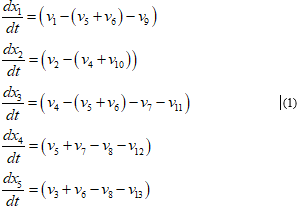
The model equations are 

Where;

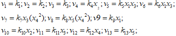
The base parameters are 

represent cholesterol, CRH, ACTH, cortisol, and aldosterone. 

Bifurcation analysis 

 The MATLAB software MATCONT is used to perform the bifurcation calculations. Bifurcation analysis deals with multiple steady-states and limit cycles. Multiple steady states occur because of the existence of branch and limit points. Hopf bifurcation points cause limit cycles. A commonly used MATLAB program that locates limit points, branch points, and Hopf bifurcation points is MATCONT (Dhooge Govearts, and Kuznetsov, 2003[29]; Dhooge Govearts, Kuznetsov, Mestrom and Riet, 2004[30]). This program detects Limit points (LP), branch points (BP), and Hopf bifurcation points(H) for an ODE system 

Let the bifurcation parameter be Since the gradient is orthogonal to the tangent vector, 

The tangent plane at any point must satisfy 

 Where A is where   is the Jacobian matrix. For both limit and branch points, the matrix  must be singular.   The n+1 th component of the tangent vector  = 0 for a limit point (LP)and for a branch point (BP) the matrix  must be singular. At a Hopf bifurcation point,                                                                  

 @ Indicates the bialternate product while  is the n-square identity matrix. Hopf bifurcations cause limit cycles and should be eliminated because limit cycles make optimization and control tasks very difficult.  More details can be found in Kuznetsov (1998 [31]; 2009 [32]) and Govaerts [2000] [33]

Hopf bifurcations cause unwanted oscillatory behavior and limit cycles. The tanh activation function (where a control value u is replaced by)   is commonly used in neural nets (Dubey et al 2022[34]; Kamalov et al, 2021[35] and Szandała, 2020[36]) and optimal control problems (Sridhar 2023[37]) to eliminate spikes in the optimal control profile.  Hopf bifurcation points cause oscillatory behavior. Oscillations are similar to spikes, and the results in Sridhar (2024) [37] demonstrate that the tanh factor also eliminates the Hopf bifurcation by preventing the occurrence of oscillations. Sridhar (2024) [38] explained with several examples how the activation factor involving the tanh function successfully eliminates the limit cycle causing Hopf bifurcation points. This was because the tanh function increases the time period of the oscillatory behavior, which occurs in the form of a limit cycle caused by Hopf bifurcations.

Multiobjective Nonlinear Model Predictive Control (MNLMPC) 

Flores Tlacuahuaz et al (2012) [39] developed a multiobjective nonlinear model predictive control (MNLMPC) method that is rigorous and does not involve weighting functions or additional constraints. This procedure is used for performing the MNLMPC calculations Here (j=12.n) represents the variables that need to be minimized/maximized simultaneously for a problem involving a set of ODE being the final time value, and n the total number of objective variables and. u the control parameter. This MNLMPC procedure first solves the single objective optimal control problem independently optimizing each of the variables   individually.  The minimization/maximization of  will lead to the values  Then the optimization problem that will be solved is This will provide the values of u at various times. The first obtained control value of u is implemented and the rest are discarded. This procedure is repeated until the implemented and the first obtained control values are the same or if the Utopia point where (  for all j) is obtained. Pyomo (Hart et al, 2017) [40] is used for these calculations.  Here, the differential equations are converted to a Nonlinear Program (NLP) using the orthogonal collocation method   The NLP is solved using IPOPT (Wächter And Biegler, 2006) [41]and confirmed as a global solution with BARON (Tawarmalani, M. and N. V. Sahinidis 2005) [42]. 

The steps of the algorithm are as follows 

1. Optimize  and obtain  at various time intervals ti. The subscript i is the index for each time step. 
2. Minimize and get the control values for various times.
3. Implement the first obtained control values 
4. Repeat steps 1 to 3 until there is an insignificant difference between the implemented and the first obtained value of the control variables or if the Utopia point is achieved. The Utopia point is when  for all j. 

When the bifurcation analysis was performed with k4 as the bifurcation parameter, a Hopf bifurcation point was located at (x1, x2x3, x4, k4) values of (0.003067, 0, 0, 0, 0, 0.815058) as shown in curve AB in Fig. 1 When k4 was modified to k4 tanh(k4)/100 the Hopf bifurcation disappears. This is shown in curve AC in Fig. 1. When the bifurcation analysis was performed with k4 as the bifurcation parameter, a Hopf bifurcation point was located at (x1, x2x3, x4, k4) values of (0.003067, 0, 0, 0, 0, 12.539816) as shown in curve AB in Fig. 2.  When k5 was modified to k5 tanh(k5)/100 the Hopf bifurcation disappears. This is shown in curve AC in Fig. 2. When k6 was the bifurcation parameter, a Hopf bifurcation point was located at (x1, x2x3, x4, k6) values of (0.003067, 0, 0, 0, 0, 2.869237) as shown in curve ABC in Fig. 3 When k6 was modified to k6 tanh(k6)/100 the Hopf bifurcation disappears. This is shown in the curve ABD in Fig. 3. 

When k11 was the bifurcation parameter, a Hopf bifurcation point was located at (x1, x2x3, x4, k11) values of (0.003067, 0, 0, 0, 0, 0.062997) as shown in curve ABC in Fig. 4 When k11 was modified to k11 tanh(k11)/650 the Hopf bifurcation disappears. This is shown in the curve ABD in Fig. 4. 

When k12 was the bifurcation parameter, two Hopf bifurcation points were located at (x1, x2x3, x4, k12) values of (0.003067, 0, 0, 0, 0, 0.400456) and (0.003067, 0, 0, 0, 0, 0.517213) as shown in curve ABC in Fig. 5 When k12 was modified to k12 tanh(k12)/0.005 the Hopf bifurcation disappears. This is shown in the curve ADC in Fig. 5. With all the bifurcation parameters, the use of the tanh activation factor was successful in eliminating the Hopf bifurcation points that cause unwanted limit cycles and oscillatory behavior validating the analysis of Sridhar (2024) [38]

For the MNLMPC calculations,

were    minimized individually and led to values of 0.135435E-02, 0, 0, and 0. k4 was the control parameter.  The multiobjective optimal control problem will involve the minimization of  subject to the equations governing the model. This led to a value of zero (the Utopia solution).   The control value k4 stayed constant at 0.05. Figure 6, 7 amd 8 show the various MNLMPC profiles.

                                                                              Figure 1: Bifurcation analysis with k4 as bifurcation parameter

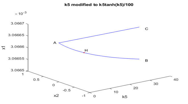
                                                                                Figure 2: Bifurcation analysis with k5 as bifurcation parameter

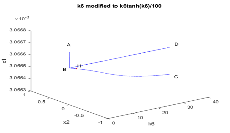
                                                                            Figure 3: Bifurcation analysis with k6 as bifurcation parameter

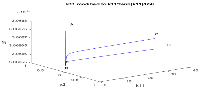
                                                                          Figure 4: Bifurcation analysis with k11 as bifurcation parameter

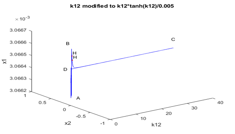
                                                                                 Figure 5: Bifurcation analysis with k12 as bifurcation parameter

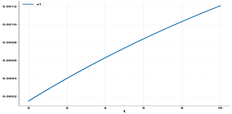
                                                                                                                  Figure 6: MNLMPC with x1 vs t

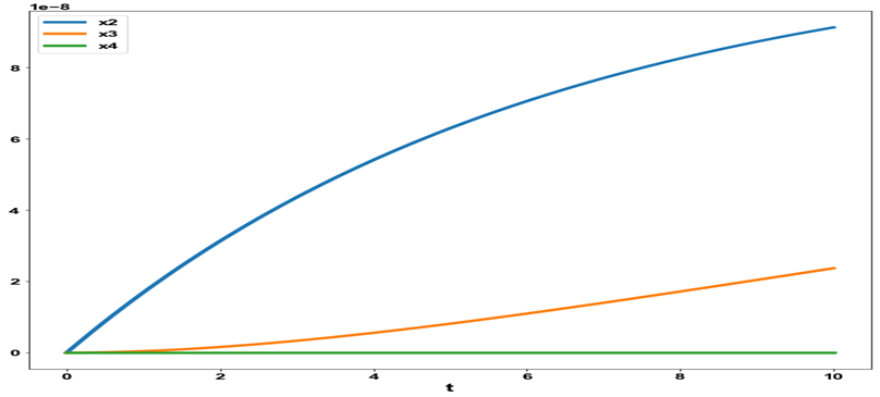
                                                                                                              Figure 7: MNLMPC with x2 x3 x4 vs t

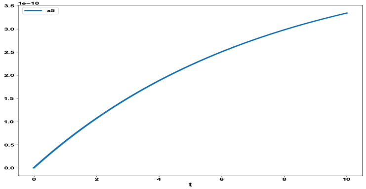
                                                                                                                  Figure 8: MNLMPC with x5 vs t

Bifurcation analysis and multiobjective nonlinear model predictive control calculations were performed on a dynamic hypothalamic-pituitary-adrenal (HPA) axis model. The bifurcation analysis revealed the existence of a limit cycle causing Hopf bifurcation points, which are eliminated using an activation factor involving the tanh function. The multi-objective nonlinear model predictive calculations converged to the Utopia point (the best possible solution). The integration of the bifurcation analysis and multiobjective nonlinear model predictive control for a dynamic hypothalamic-pituitary-adrenal (HPA) axis model is the main contribution of this paper.

All data used is presented in the paper

The author, Dr. Lakshmi N Sridhar has no conflict of interest.

Dr. Sridhar thanks Dr. Carlos Ramirez and Dr. Suleiman for encouraging him to write single-author papers.