A method is developed to allow cardiologists to find changes in the blood flow rate in larger coronary arteries, caused by the appearance of their pathological tortuosity, and a hemodynamic significance of those changes based on the data taken from the appropriate coronarographies only. This method is based on replacement of blood flows in the originally healthy and subsequently pathologically tortuous artery with the corresponding averaged ones, and subsequent calculation of flow characteristics of interest in terms of the corresponding averaged flow characteristics. It allows one not to take account of a number of identical factors for the originally healthy and subsequently pathologically tortuous segment of the investigated artery, and gives one the possibility to determine the flow parameters of concern at any time after carrying out a coronarography. In addition, it is not associated with solving complicated technical problems, and does not require special facility to be used, special professional training and significant financial and temporal expenses. The method was successfully tested in-vitro and then applied to appropriate patients. It was found that the hemodynamic significance of the tortuosity generally increases/decreases as the number of the tortuosity arcs increases/decreases. Also, strong correlation between fundamental geometric and hemodynamic characteristics of the tortuosity and basic clinical indicators of the corresponding patients was established. This suggests a strong independent influence of the tortuosity on the clinical symptoms of the corresponding patients. The critical values for the number of the tortuosity arcs, the relative blood flow rate loss and the rate of angina pectoris attacks were obtained, starting from which the corresponding tortuosity can be hemodynamically significant.

                               height of the i-th tortuosity arc

    covariance of appropriate magnitudes

                              cross-sectional diameter of a normal coronary artery

                             cross-sectional diameter of a tortuous arterial segment

                width of the i-th tortuosity arc

                              axial dimension of a tortuous segment

                            length of the straight segment of a conditionally normal coronary artery

                               length of the i-th tortuosity arc

                              length of a tortuous arterial segment

                               the number of appropriate patients/tortuosities

               the number of arcs in a tortuous coronary artery

                              the number of the tortuosity arcs starting from which the corresponding tortuosity can be hemodynamically significant

                rate of angina pectoris attacks

                               rate of angina pectoris attacks corresponding to

                blood flow rate

                              blood flow rate in a normal coronary artery

                             blood flow rate in a tortuous coronary artery

                             blood flow rate loss in a coronary artery due to its pathological tortuosity

                               correlation coefficient between appropriate magnitudes

                              significance of the coefficient

                             critical value for

                               time needed for blood to pass the straight segment of a normal coronary artery

                              time needed for blood to pass the tortuous arterial segment

                              mean (cross-sectionally averaged) axial blood flow velocity in a normal coronary artery

                             mean (cross-sectionally averaged) axial blood flow velocity in a tortuous coronary artery

                             loss in the mean axial blood flow velocity in a coronary artery due to its pathological tortuosity

                significance level

                              relative loss in the blood flow rate in a coronary artery due to its pathological tortuosity ensemble-averaged relative loss in the blood flow rate in a coronary artery due to its pathological tortuosity

                             critical value for

                              relative blood flow rate loss in a tortuosity corresponding to arcs

                              relative loss in the mean axial blood flow velocity in a coronary artery due to its pathological tortuosity

                              ensemble-averaged relative loss in the mean axial blood flow velocity in a coronary artery due to its pathological tortuosity

                               sample mean of the magnitude

                              dispersion of the magnitude

                              mean-square deviation of the magnitude

AIVB                         anterior interventricular branch

CA                              coronary artery

CAG                           coronary angiography

CSX                           cardiac syndrome X

FC                              functional class of patients

IHD                            ischemic heart disease

LCA                           left coronary artery

MI                              myocardial ischemia

RCA                           right coronary artery

SCAT                         severe coronary artery tortuosity

Coronary arteries (CAs) are the vessels supplying myocardium with an oxygen-rich blood. They are the only sources of blood supply to the myocardium, and are situated both on the heart surface and within the myocardium constituting the so-called coronary tree. In this tree, there are the two main branches. These are the left branch (usually called the left coronary artery (LCA)) and the right one (ordinary referred to as the right coronary artery (RCA)).

The most severe and the most widely spread disease of coronary arteries is atherosclerosis. It is accompanied by depositing cholesterins and some fractions of lipoproteins on the inner surface of the vessel wall, with their subsequent calcification. As a result, in such coronary arteries fast local narrowings (i.e., stenoses) are formed, which, apart from the others, result in the blood flow reduction in the arteries and possible further development of myocardial ischemia (MI).

Until quite recently, stenoses were considered to be the only reason for the appearance and development MI. However, numerous latest investigations (see, for example, [1-10]) show that in approximately 7-30% of patients with the common symptoms of MI one cannot detect stenoses in their coronary arteries (such a phenomenon (i.e., the availability of the common symptoms of MI in patients with non-stenosed CAs) was called the cardiac syndrome X [3, 4, 6, 7]). At the same time, in the coronarograms of approximately more than 75% of these patients, larger coronary arteries (i.e., the arteries whose diameter exceeds approximately 0.5 mm) with a severe pathological tortuosity are clearly observed [3, 4, 6, 7, 10-15] (Figure 1).

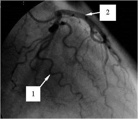
Figure 1: Coronarogram of the LCA with a severe pathological tortuosity of a few larger arteries.

According to the opinion of the dominant majority of researchers (see, for example, [3-15]), this tortuosity is the main reason for the appearance of the noted syndrome. It is explained by the fact that the appearance of a pathological tortuosity in the originally normal (usually straight) segment of a coronary artery results in (i) an increase in the segment resistance to the blood motion; (ii) an additional pressure drop in the segment; (iii) an increase of the distance passed by blood in the segment and the corresponding increase of the viscous forces’ influence on the flow there, and hence, an increase in the blood flow energy dissipation, etc. All of these factors inevitably cause (apart from the other effects) a decrease in the blood flow velocity and rate in the coronary artery, and, under the appropriate circumstances, subsequent possible development of cardiac ischemia.

The discovery of the cardiac syndrome X and the ascertainment of the main reason for its initiation have stimulated researchers to make the corresponding investigations. In those investigations, various aspects of fluid motion in channels with local tortuosity were studied. However, despite of the significant results obtained in those studies, for the moment no methods have been developed that would allow cardiologists to determine (with satisfactory precision and speed)

• the changes in the blood flow characteristics of interest in larger coronary arteries, which are caused by the appearance of their pathological tortuosity.
• the hemodynamic significance of those changes based on the data taken from the appropriate coronarographies only.

The available methods of diagnosis of hemodynamic significance of anatomic changes in segments of the coronary tree are usually either low efficient or their application is technically impossible in case of a severe coronary artery tortuosity (SCAT).

This disadvantage is partly corrected in the present paper. Here an approximate method is developed that allows cardiologists to find (with satisfactory precision and speed) both the above-noted changes in the blood flow characteristics of interest and the hemodynamic significance of those changes proceed from the information obtained from the appropriate coronarographies only. This method is based on replacement of real blood flows in the originally healthy and subsequently pathologically tortuous coronary artery with the corresponding cross-sectionally averaged ones, subsequent obtaining the blood flow characteristics of interest in terms of the corresponding averaged flow characteristics and making a comparative analysis of the appropriate obtained flow characteristics with one another. Apart from this, the method allows one not to take account of a number of identical factors for the originally healthy and subsequently pathologically tortuous segment of the coronary artery under investigation, and gives one the possibility to determine the blood flow parameters of concern at any time after carrying out a coronarography. In addition, the developed method is not associated with solving complicated technical problems, and does not require special facility to be used, special professional training and significant temporal and financial expenses.

The paper consists of an introduction, six sections, acknowledgments, a list of references and nomenclature. It begins with a formulation of the problem and a description of the corresponding model of a larger coronary artery, as well as a discussion of the considerations and assumptions made in the model development (Section 2). Then the approximate solution to the formulated problem is given (Section 3), and the method is developed on the basis of that solution (Section 4). Section 5 presents the results of the laboratory experiment in which the method is tested. The results of application of the method to the appropriate patients are described and analyzed in Section 6. After that the conclusions of the investigation are set out (Section 7), and acknowledgments are given. Finally, lists of the literature cited and notations used in the paper are presented.

2.1. The problem and the model

An arbitrary larger coronary artery is considered, that initially is in the normal state. In some time, a severe pathological tortuosity appears in its finite (usually straight) segment. It is necessary, based on the data obtained from the appropriate coronarography only, to find changes in the blood flow characteristics of interest in the artery caused by that tortuosity and determine a hemodynamic significance of those changes with satisfactory for cardiologists’ precision and speed.

Figure 2 presents the corresponding model of the normal coronary artery and that of the artery having already a pathologically tortuous segment of axial dimension (usually, this dimension ranges approximately from 3 mm to 10 mm). In the first case, the artery is represented by an infinite straight rigid pipe, of circular cross-section of diameter, in which fluid (blood) flows. The fluid motion is characterized by the flow rate (which is so far unknown). In the second case, the artery is modelled by an infinite straight hard-walled pipe having circular cross-section of constant diameter (, )2 and a finite tortuous segment. This segment has   arcs (which are its parts between the two neighbouring points of its wall intersection with the dashed line (this line corresponds to the pipe wall position before the appearance of the tortuosity)). Each arc is characterized by height (which is the maximal distance from its wall to the dashed line) and width (this is the distance between its ends) (). The moving fluid in this pipe has the flow rate (which is also so far unknown).

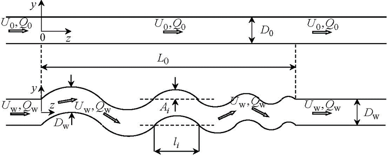
Figure 2: Originally straight and subsequently pathologically tortuous segment of a coronary artery.

The considerations and the assumptions used in developing this model are given below.

2.2. The considerations and the assumptions

2.2.1. Larger coronary artery

Larger coronary artery in a normal state actually is a finite nearly straight slightly taper (in the flow direction) elastic pipe having nearly circular cross-section. However, in this study the artery is modelled by an infinite straight rigid-walled pipe of constant (along its axis) circular cross-sectional shape and area. Such a representation of the artery is mainly for the following two reasons. Firstly, consideration of an infinite pipe (instead of a finite one), with the given typical flow parameter values at infinity, allows one to determine (with satisfactory for cardiologist’s precision) the flow characteristics of interest in the vessel segment under consideration and not to pay attention to what is upstream and downstream of that segment. Secondly, it is clear that, at the chosen precision of the investigation (see the end of the Introduction and the very beginning of this section), the neglect of both the insignificant deflection of the arterial cross-sectional shape from the circular one and the slight arterial tape redness will not have a principal influence on the results and the conclusions of this study. As for the arterial wall compliance and its influence on the inner blood flow, as well as the arterial fastening in the ambient medium and the ambient medium effects, etc., all of them (together with those noted above) are indirectly taken account of in the model (via the blood velocity which is found from the corresponding coronarographies containing all the information of interest (see Section 6)).

2.2.2. Pathologically tortuous arterial segment

The appearance of pathological tortuosity in some arterial segment is accompanied by its non-significant narrowing2. This is taken into account in the model shown in Fig. 2 via the diameter Dw, which is slightly smaller than the diameter D0.

2.2.3. Blood

As in the dominant majority of the appropriate investigations (see, for example, [15, 19-23]), in this study blood is assumed to be an incompressible, homogeneous and Newtonian fluid. The first assumption is based on the fact that the blood flow velocities are small values compared to the sound speed in blood. The second assumption is due to practically 

homogeneous distribution of all the constructive elements of normal blood in its plasma, and the third one is valid at high shear rates above 

approximately 50s-1, commonly found in the larger coronary arteries [19-23]. As for possible deflection in values of these blood characteristics from the above noted ones, as well as the other features of blood rheology (such as dependence of the blood mass density and viscosity on the body temperature, etc.), they are indirectly taken account of in the developed model. Again, it is made via the blood flow velocity (see Subsection 2.2.1).

2.2.4. Flow

Real blood flow is pulsatile, having the pulsation frequency and time period of the order of 1Hz and 1s, respectively. However, in the model, one actually restricts oneself to the consideration of quasi-steady flow, whose integral characteristics coincide with the corresponding characteristics of real blood flow observable in patients. Also, the model flow is assumed to be a laminar. The former restriction is explained by the fact that at this stage only the blood volume reaching a myocardium during the heartbeat period is of urgent interest rather than how that volume varies over the period. As for the later assumption, it reflects the reality quite well, because usually real blood flow is laminar. If nevertheless it is disturbed (or even becomes turbulent) in some vessel segment, then, due to the absence of the corresponding perturbation sources and the permanent influence of viscous forces on the flow behind the segment, the flow disturbances (turbulisation) vanish rather fast, and the flow redevelops back to the state upstream of the segment [19-23]. (Here attention should be also paid to the following two circumstances. Firstly, due to the accuracy accepted in this study (see above), the quasi-steady and laminar approximations to real blood flow are not very principal for the results and the conclusions of this study. This is due to that (as one can see in Section 6) (i) the time intervals (over which a Roentgen-contrast fluid passes through the coronary artery segments of concern) will be significantly smaller than the time scale of the problem under consideration (i.e., the heartbeat period), which makes the flow variation over the intervals not a very significant factor; (ii) the solution to the problem will be obtained in terms of the flow characteristics averaged in the appropriate manner, which significantly reduces the difference between the model and real flows. And secondly, the real blood flow character and regime are nevertheless taken account of indirectly in the model shown in Figure 2. As in the cases of the other constructive elements of the model (see above), it is made via the blood flow velocity, which is found from the appropriate coronarographies.)

3.1. General relationships

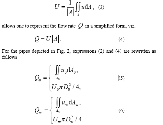
Since among all the blood flow dynamical characteristics the most important for normal functioning of the myocardium are the blood flow rate and cross-sectionally averaged axial velocity, these characteristics are paid the main attention to in this study. If the blood volume passing across some vessel cross-section, , over a small time interval is denoted by (where is the axis chosen in Fig. 2), then the blood flow rate in that section, , is found as the ratio of and , viz.

.                       (1)

If one takes into account that the volume is found as the integral of the local axial blood flow velocity, , over the section, viz.

,

the magnitude in (1) can be represented by the following integral

.                              (2)

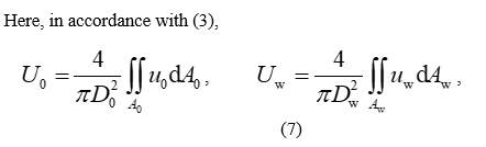
On the other hand, the multiplication and division of the right part of [removed]2) by (where is the area of the section ) and taking account of the fact that the ratio of the integral and is the cross-sectionally averaged (mean) axial blood flow velocity, , in the section , viz.

and hereinafter the indices “0” and “w” indicate the normal and tortuous vessel, respectively.

Theoretically, relationships (5)-(7) give one the possibility to find (in the framework of the model described in Section 2) the blood flow rate and the cross-sectionally averaged (mean) axial blood flow velocity in the originally normal and subsequently pathologically tortuous segment of the artery under investigation, and then, based on the expressions

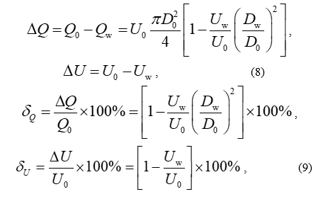
find the absolute (8) and relative (9) changes in these flow characteristics, which are caused by the appearance of the noted tortuosity. However, as one can see from the analysis of formulas (5)-(9), these mathematical operations can be only made under the availability of a complete and reliable information about the corresponding local (i.e., , ) and/or mean (i.e., , ) axial blood flow velocities.

This information can be obtained by the two methods. The first of them is based on direct numerical modelling of the flow in the arterial segment under consideration, with taking account of all the rheological features of blood, properties of the arterial wall and its fastening, the blood-wall interaction, etc. It allows one to find rather accurately the velocities and , and hence, the magnitudes , and , . However, this approach is associated with significanttemporal and financial expenses, which is undesirable (because patients prefer to have fast and cheap diagnostics, and cardiologists need to make fast (or even immediate) and correct decision about the patient state). Therefore, so far it is unacceptable.

The second method (its description is given in Subsection 3.2) is in an approximate experimental determination of the mean axial blood flow velocities and (proceed from the appropriate data obtained from the corresponding coronarographies), with subsequent computation of the blood flow rates and based on the lower expressions in (5) and (6). Herewith the blood rheology, the arterial wall properties and the artery fastening in the ambient medium, as well as the blood-wall interaction, etc. are taken account of automatically from the corresponding coronarographies. This approach does not need significant temporal (maximum a couple of hours for making a decision) and financial expenses, its precision is satisfactory for cardiologists, and hence, for the moment it is more acceptable for them compared to the first method.

Proceed from the just-noted, further in this paper the second approach is chosen to find the velocities and , and consequently, the flow rates and , as well as the absolute and relative changes in these flow characteristics.

3.2. An approximate experimental method to find and

Before proceeding to description of this method, let us pay our attention to one important physical feature of mathematically equivalent expressions (2) and (4), as well as the consequences resulting from that feature. The matter is that the formal transition from (2) to (4) on the basis of (3) means not only the transition from the local, , to averaged, , axial flow velocity but also (that is much more important) the transition from the consideration of real to the averaged, in the appropriate manner, flow (because the averaged flow velocity is a velocity of the appropriately averaged flow). Further in a cross-sectionally averaged (quasi-steady) laminar flow (such a flow is actually observed by cardiologists when studying coronarographies (see also Subsection 2.2.4)) the velocities of all fluid particles are equal vectors (Fig. 3), and the particles’ trajectories, therefore, are identical curves which have the same length [24]. Apart from the others, it means that in such a flow in vessel

• the trajectories of all fluid particles are like the vessel axis;
• the distance covered by the particles during some time is equal to the length of the corresponding axial segment;

the fluid particle velocity (i.e., the mean axial flow velocity, ) is determined as the ratio of the distance and the time , viz.

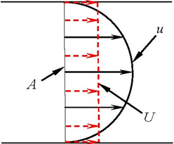
Figure 3: Schematic profiles of the velocities and in a laminar pipe flow.

The above considerations allow one to determine approximately the velocities and based on the appropriate data obtained from the corresponding coronarography (CAG) only and formula (10). The corresponding general procedure of finding the noted velocities reduces to the following three main steps, viz.

• determination of the distance covered by the Roentgen-contrast fluid front together with blood in the arterial segment under investigation proceed from the appropriate data taken from the corresponding CAG;
• finding the time interval , during which the above-noted front passes the distance , based on the number of corresponding picture areas of the investigated CAG and the time duration of one picture area;
• calculation of the blood flow velocity of concern on the basis of the above data for and , as well as formula (10).

For the originally normal and subsequently pathologically tortuous segment of a larger coronary artery, these steps can be realized in the following way.

Originally normal arterial segment.

The length of the originally normal arterial segment (Fig. 2) and the time , during which the front of a Roentgen-contrast fluid passes through the segment (i.e., covers the distance ), are found from the chosen CAG by direct measuring and counting (proceed from the number of the corresponding picture areas and the time duration of one picture area), respectively. Then the velocity is calculated from the ratio

.                      (11)

Pathologically tortuous arterial segment.

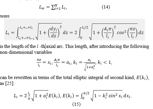
The distance covered by the Roentgen-contrast fluid front, when it passes through the tortuous arterial segment (Figs. 1 and 2), is equal to the length of the segment axis (the corresponding arguments are given before [removed]10)). Since the axis has the shape of an irregular sinusoid, it is logically to approximate the segment axis by such a sinusoid (Figure 4), viz.

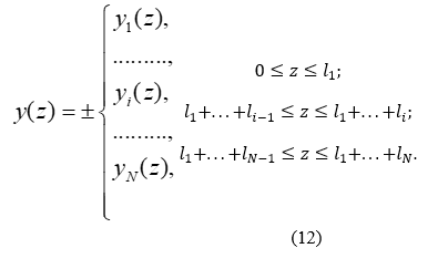
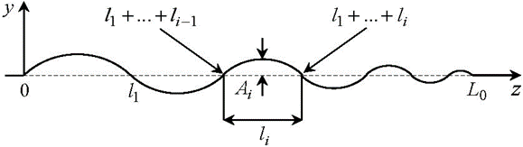
Figure 4: The tortuous segment axis approximated by an irregular sinusoid.

Here () are ordinary sine functions in the indicated domains, viz.

which approximate the axes of the corresponding arcs, the magnitudes and are their heights and widths, respectively, (they are measured directly from the corresponding coronarogramm, and are identical to those shown in Fig. 2) and the plus-minus signs indicate the cases when the first arc is either above or below the -axis, respectively.

In such a situation, the distance can obviously be found as the length of the curve (12), (13), viz.

The availability of the distance (14) and the time needed for the front of a Roentgen-contrast fluid to cover that distance (is found from the investigated CAG by direct counting the number of the corresponding picture areas and subsequent multiplying that number by the time duration of one picture area) allows one to find the velocity as the ratio of and , viz.

The considerations presented, as well as the results and the relationships obtained in Sections 2 and 3 allow one to suggest the following approximate method to diagnose the hemodynamic significance of a pathological tortuosity of larger coronary arteries in patients with myocardial ischemia (MI), cardiac syndrome X (CSX) and severe coronary artery tortuosity (SCAT).

1. When the patient exhibits the common symptoms of MI (such as chest pain (typically on the left side of the body), neck or jaw pain, shoulder or arm pain, a fast heartbeat, shortness of breath when he/she is physically active, extreme fatigue and sweat secretion, etc.), his/her coronary angiography (CAG) is carried out.
2. If the obtained CAG does not exhibit stenoses in coronary arteries (CA) and at least one coronary artery has a segment with SCAT, then the segment cross-sectional diameter, , as well as the height, , and the width, , of each segment arc (; Fig. 2) are determined from the CAG by direct measuring.
3. Based on the found values of and the axis of the investigated tortuous segment is approximated by the irregular sinusoid (12), (13).
4. Based on relationships (14) and (15), as well as the tables of the total elliptic integral of second kind [25], the axis length (i.e., the distance covered by the Roentgen-contrast fluid front when moving together with blood through the segment) is found.
5. The time , needed for the front to cover the distance , is determined from the investigated CAG as the product of the number of the corresponding picture areas and the time duration of one picture area.
6. The mean axial blood flow velocity in the investigated tortuous segment is found from [removed]16).
7. As the originally normal coronary artery (i.e., the investigated artery before the appearance of the tortuosity in it) an artery without pathological tortuosity is chosen in the same CAG[1]. Its cross-sectional dimension, , should be slightly larger than the diameter (i.e., , )2. In this artery, a straight segment (or, in case of absence of a straight segment, a segment whose shape is maximally close to the straight one) is further considered, whose length, , is close to the axial dimension of the investigated tortuous segment, (i.e., , Fig. 2)[2].
8. Based on the number of the corresponding picture areas and the time duration of one picture area (which are taken from the used CAG), the time , needed for the front of a Roentgen-contrast fluid to cover the chosen straight segment of the conditionally normal coronary artery (i.e., the distance ), is found as the product of the above number and the time duration.
9. The mean axial blood flow velocity in this straight arterial segment, , is determined on the basis of [removed]11), where is replaced by.
10. Based on the above data and the lower expressions in (5) and (6), the blood flow rates in the conditionally normal, , and subsequently pathologically tortuous, , arterial segments are calculated.
11. Based on relationships (8) and (9), the absolute and relative changes in the corresponding blood flow characteristics in the coronary artery under investigation, which are caused by the appearance of the pathological tortuosity in it, are found.
12. The hemodynamic significance of those changes is determined, the changes being considered to be hemodynamically significant when the relative blood flow rate loss, , is not less than the corresponding critical value, (i.e., ). In the opposite case (i.e., when ) the changes are hemodynamically insignificant (the value corresponds to the 25% drop in the blood pressure in vessel due to a stenosis, which is hemodynamically significant according to the FFR method3).

5.1. Experimental System

In order to verify the above-described method before its application to appropriate patients, it has been tested in a laboratory experiment. For this purpose, a suitable experimental system has been developed. A schematic of this system and its test section is shown in Figs. 5 and 6, respectively. Here the basic elements are:

1. a couple of the upper supply and a couple of the lower collection identical reservoirs;
2. ttwo identical silicone pipes, of inner diameter mm, , representing an originally healthy and subsequently pathologically tortuous larger coronary artery (see below the explanation of how the pipe shape was fixed);
3. measuring reels to measure the pipes’ geometrical parameters of interest;
4. needles (for dye injection) flush-mounted into the pipe wall upstream of the test section;
5. a video camera to record the dye motion in the pipes;
6. transparent glue ribbon to fix the pipe shape of interest;
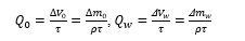
7. two electronic balances to determine the fluid volumes accumulated in the collection reservoirs during the period of data acquisition, , based on the formula

(here and are the corresponding water volumes accumulated in the collection reservoirs during the time [1]).  Then the found data for and and the lower expressions in (5), (6) were used to compute the corresponding velocities and , viz.[2] 

(where  and  are the volume and the mass of fluid, respectively passed to the appropriate reservoir during the time , and  the fluid mass density). (Also, the magnitude could could be found visually by direct measuring the corresponding fluid volume that passed to the collection reservoir, calibrated in liters, during the time .. However, due to relatively small volumes  and rather big cross-sectional area of the reservoir, the corresponding changes in the water levels in it were so small that the accuracy of these measurements was lower than the accuracy of the corresponding data obtained on the basis of relationship (17).)

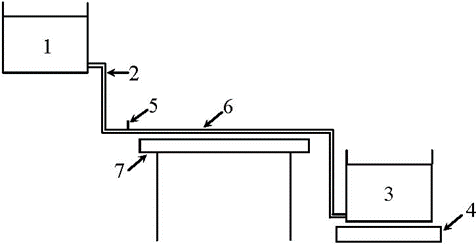
Figure 5: Schematic of experimental system: 1 – supply reservoir; 2 – silicone pipe; 3 – collection reservoir; 4 - electronic balance; 5 – needle for dye injection; 6 – test section; 7 – table.

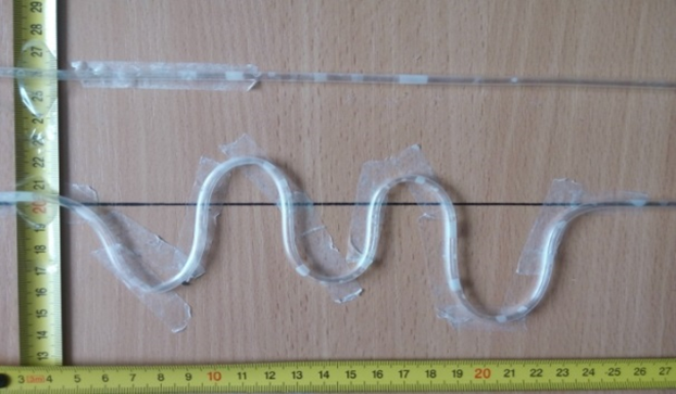
Figure 6: Test section.

The working medium was water at an indoor temperature (the considerations and the assumptions used in developing the test section were like those given in Subsection 2.2 and in [20-22]).

The experimental system was operated in the following way. The upper and lower tanks were joined by the pipes (one pipe per one set of the upper and lower tanks, see Figure 5). One pipe was straight and represented an originally healthy coronary artery. Another one had a tortuous segment, with all the adjusted geometrical parameters of concern (due to pipe flattening, that took place at the tortuosity apices at some ratios of the arcs’ heights and widths, , those ratios were not considered in the experiment). It simulated a tortuous coronary artery. Due to the same levels of water in the corresponding reservoirs, a controlled flow with identical pressure gradients was created in each pipe. A similarity in the flow Reynolds number, , (based on the mean axial flow velocity in vessel and the inner vessel diameter) between the experimental flow and real blood flow observable in the appropriate coronary arteries in the patients was held herewith (for all the patients used in this study (see Section 6), the number did not exceed 1800, that indicated that the flow in the coronary arteries of interest and the experimental flow were always laminar [24]). Mild dye injection into the pipes via the needles situated immediately upstream of the test section allowed one to visualize the flows and make their video-records.

For these experimental flows, their mean axial velocities, and , and the corresponding flow rates, and , were determined on the basis of the method described in Section 4. Then these data were compared with the corresponding reference data. After that, proceed from the results of such a comparison and the corresponding discussions with the cardiologists, a conclusion concerning the applicability of the method to appropriate patients was made.

The reference data were obtained on the basis of the corresponding measurements. More specifically, initially the water masses, passed simultaneously from the straight, , and tortuous, , pipes to the  appropriate collection reservoirs during the period , were measured by means of the electronic balances. It allowed one to find the flow rates in the pipes, and , from relationships (1) and (17), viz.

(here and are the corresponding water volumes accumulated in the collection reservoirs during the time [1]).  Then the found data for and and the lower expressions in (5), (6) were used to compute the corresponding velocities and , viz.[2] 

5.3. Experimental Results

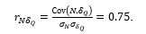
Some typical results of such a comparison, obtained for the pipes’ configurations shown in Fig. 6, are presented below. Here the axial dimension of the tortuous segment, , and the number of its arcs, , were chosen to be 200mm and 5, respectively, and the values of the arcs’ heights, , and widths, , () were as those given in Table 1. With these magnitudes available and in accordance with the method described in Section 4, the tortuous segment axis was then approximated by the irregular sinusoid (12), (13). Further application of relationships (14) and (15), as well as the use of the above magnitudes and the tables of the total elliptic integral of second kind [25] allowed one to find both the lengths of the axial arcs (Table 1) and the length of the tortuous segment axis (i.e., the distance covered by the dye when it moved through the segment), viz. mm.
covered by the dye when it moved through the segment), viz. mm

	1	2	3	4
	37	19	34	10	49
	48	31	33	27	61
	92	51	77	35	120

Table 1. Values (in mm) of the tortuosity parameters in Figure. 6.

The availability of the distances and , as well as the corresponding time intervals s and s (found by the way indicated in the method) gave one (on the basis of expressions (11) and (16)) the values of the mean axial flow velocities in the straight, , and tortuous, , pipe segments, viz.

Then the magnitudes (18) allowed one to determine (proceed from the lower expressions in (5) and (6)) the corresponding flow rates and , viz.

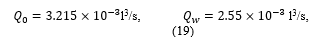
and the corresponding absolute and relative losses in these flow characteristics, viz.

which are caused by the appearance of the tortuosity.

The comparative analysis of the values (18)-(20) with the corresponding reference data, viz.

(found in the manner described above) showed rather good agreement between them. Also, this agreement was acceptable for the cardiologists.

Similar results of the comparison (i.e., within 10% of the corresponding relative differences) have also been obtained for all the other tortuosity configurations used in this experiment. From this and the corresponding discussions with the cardiologists, one has come to the conclusion that the method described in Section 4 gave one the results which were acceptable for cardiologists and hence, it could be applied 

6.1. Selection of patients for the investigation

After the successful laboratory verification of the method, it was further applied in the cardiological and cardio-surgical departments of the city hospital no 9 (Odessa, Ukraine) and the department of interventional cardiology of the Saint Catherine’s cardiological clinic (Odessa, Ukraine). Here among 3234 investigated patients with the common symptoms of ischemic heart disease (IHD) and coronary angiographies (CAGs) made, 217 ones (6.71%) had the cardiac syndrome X (CSX), and in 148 patients of the later ones (68.2%) a severe pathological tortuosity of larger epicardial coronary arteries was found. Herewith 49 patients of them (33.11%) had only one CA affected by the tortuosity, whereas in the CAGs of the other 99 ones (66.89%) a severe tortuosity of two or three CAs was clearly observed (Table 2). The number of arcs in their tortuous arteries ranged from 2 to 9 (i.e., ).

Table 2: Larger coronary arteries affected by the tortuosity in the patients with IHD, CSX and SCAT.

Apart from these, 23 patients with SCAT (15.5%) had arterial involvements of the noted kind in two branches of the left coronary artery (LCA; see Table 2), coronarographies of 12 patients with SCAT (8.2%) exhibited the tortuosity of one branch in the LCA and one branch in the RCA, and 64 patients of the chosen 148 ones (43.2%) had three larger CAs affected by the tortuosity.

Further analysis of the patients with SCAT has shown that the dominant majority of them (i.e., 112 ones (75.7%)) had arterial involvements of such kind in the anterior interventricular branch (AIVB) of the LCA (see Table 2). In addition, this branch was the most severely affected by the tortuosity among all the other coronary arteries in all the investigated patients with SCAT. Since, according to the data available in the scientific literature (see, for example, [11-13, 26-28]), the AIVB of the LCA also is most often and severely affected by the pathological tortuosity, the noted 112 patients were selected for further investigation by the method described in Section 4, as well as by the other appropriate procedures to decide on hemodynamic significance or insignificance of their SCAT, etc.

Below an example of application of the method to the patient, whose coronarogram is shown in Fig. 1 (this is a standard left skew cranial projection), is given.

6.2. Example of clinical application of the method

In this subsection, one demonstrates an application of the method to the patient, whose coronarogram is shown in Fig. 1. In this patient, by means of making appropriate physical exercises, the common symptoms of IHD were detected, and accordingly, the coronarography (CAG) was carried out (item (a) of the method, see Section 4). In this CAG, senoses were absent. However, one larger coronary artery, having a segment with a severe pathological tortuosity, was observed (the artery is denoted by number 1 in Figure 1; this is the AIVB of the LCA). This segment had 9 arcs (i.e., ), its cross-sectional diameter, , found from the CAG by direct measurement, was equal to 1.7mm, and the values of the heights, , and the widths, , of all its arcs, also found from the CAG by direct measurement, are given in Table 3 (item (b) of the method).

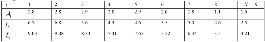
Table 3: Values (in mm) of the geometrical parameters of the tortuous arterial segment 1 in Figure 1.

The availability of values of and allows one (in accordance with items (c) and (d) of the method)

• to approximate the axis of the tortuous segment by the irregular sinusoid (12), (13);
• to determine the lengths (Table 3) of all the axial arcs based on formula (15) and the tables of the total elliptic integral of second kind [25];
• to find the distance , which is covered by blood when moving through the segment, proceed from relationship (14), viz.

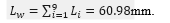
Then the found distance and the time (s)[1], which is needed for blood to pass the distance, allow one to determine the mean axial blood flow velocity, , in the discussed segment proceed from [removed]16), viz. mm/s (items (e) and (f) of the method).

Further, in accordance with item (g) of the method, the artery without pathological tortuosity, having almost straight segment of length mm, is chosen in the same CAG as the originally normal coronary artery (it is denoted by number 2 in Fig. 1; this is the envelope branch of the LCA in the proximal-middle segment in the standard straight caudal projection; for the convenience of making the investigation, it was re-projected by the cardiologists to the standard left skew cranial projection shown in Figure 1)[2]. The cross-sectional diameter of this segment, , is equal to 1.8mm ().

The chosen segment is covered by a Roentgen-contrast fluid during passing only one picture area. Since the time duration of one picture area is10 0.1s, the time , required for the fluid to pass the distance , is equal to 0.1s (item (h) of the method), and hence, in accordance with item (i) of the method, the mean axial flow velocity in the segment is equal to 195 mm/s (i.e., mm/s).

The availability of the velocities and , as well as the diameters and allows one

• to determine the blood flow rates in the originally normal, , and subsequently pathologically tortuous, , segment of the investigated coronary artery based on the lower expressions in (5) and (6) (item (j) of the method), viz. l3/s, l3/s;
• to find the absolute and relative changes both in the mean axial flow velocity and the flow rate in this artery proceed from expressions (8) and (9), which are caused by the appearance of the pathological tortuosity in the artery (item (k) of the method), viz. mm/s, l3/s, , .

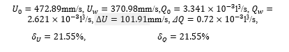
Then the comparison of the obtained value of the relative blood flow rate loss, , with the corresponding critical one, , shows that these changes are hemodynamically significant (item (l) of the method), viz. .

6.3. Results

Apart from making decision about hemodynamic significance/insignificance of pathologically tortuous coronary arteries in the selected 112 patients (see Subsection 6.1) on the basis of the method, also it was interesting to get answers to the following questions of practical and scientific interest.

1. How does the hemodynamic significance/insignificance of the SCAT depend on the number of the tortuosity arcs, , the arcs’ heights, , and widths, , their ratios, , etc. ()?
2. What is the correlation between (i) the tortuosity severity[1] and the blood flow rate loss, (ii) the tortuosity severity and the rate of angina pectoris attacks, (iii) the blood flow rate loss and the rate of angina pectoris attacks, (iv) the tortuosity severity and the functional class of patients, (v) the blood flow rate loss and the functional class of patients for the investigated tortuosities?
3. What are the critical values for the number of the tortuosity arcs, the relative blood flow rate loss and the rate of angina pectoris attacks starting from which the corresponding coronary artery tortuosity can be hemodynamically significant?
4. Is it possible to conclude about strong independent influence of the coronary artery tortuosity on the clinical symptoms of patients with IHD, CSX and SCAT?
5. Is it possible, proceed from the results obtained on the basis of the method, to recommend the method for future application in clinical practice?

Below the corresponding data obtained in the selected 112 patients in the framework of the method are presented and analyzed. We begin with

1. analyzing the correlation between the relative losses in both the mean axial blood flow velocity, , and the blood flow rate, , in the AIVB of the LCA in the above patients, due to its pathological tortuosity, and the number of the tortuosity arcs, ;
2. subsequent concluding about hemodynamic significance/insignificance of these tortuosities proceeds from comparison of the corresponding values of with the critical one, , (see item (l) of the method).

In making this, the data of Tables 4-6 are used5. Herewith the ensemble-averagedrelative losses in the mean axial blood flow velocity, , and the blood flow rate, , (which are presented in Table 4) are found as arithmetic mean of the losses and , respectively over the number of the corresponding tortuosities.

	3	4	5	6	7	8	9	Total
	4	18	21	23	21	16	9	112
, %	28.69 ± 1.79	33.78 ± 0.92	42.52 ± 2.33	46.24 ± 1.67	50.63 ± 1.62	55.48 ± 2.04	60.30 ± 2.39	45.38 1.82
, %	31.73 ± 3.16	34.69 ± 1.30	44.32 ± 2.47	47.79 ± 1.52	53.08 ± 1.63	57.59 ± 1.62	62.20 ± 3.30	47.34 2.14

Table 4: Correlation between , and in the selected patients with SCAT of the AIVB of the LCA.

	3	4	5	6	7	8	9	Total
The number of patients with hemodynamically insignificant tortuosity (), n1 (%)	4 (100)	15 (83.3)	9 (42.9)	3 (13.0)	1 (4.8)	0	0	32 (28.6)
The number of patients with hemodynamically significant tortuosity (), n2 (%)	0	3 (16.7)	12 (57.1)	20 (87.0)	20 (95.2)	16 (100)	9 (100)	80 (71.4)
The total number of patients, n=n1+n2	4	18	21	23	21	16	9	112

Table 5: Correlation between the selected patients with hemodynamically insignificant/significant tortuosity and the number of the tortuosity arcs, ..

Table 6: Distribution of the selected patients with SCAT of the AIVB of the LCA vs and .

One can see from Table 4 that, on average, among all the considered tortuosities, the hemodynamically significant are those having 5 and more arcs, whereas the tortuosities with 3 and 4 arcs are hemodynamically insignificant. However, the analysis of the relative blood flow rate loss in each tortuous CA, , shows that (see Tables 5 and 6)

• there are some hemodynamically insignificant tortuosities with 5, 6 and 7 arcs;
• a few tortuous arteries having 4 arcs are hemodynamically significant.

Further analysis of Tables 4-6 indicates that, according to the method,

• 71.4% of the investigated tortuosities of the AIVB of the LCA are hemodynamically significant;
• the hemodynamic significance of the tortuosity generally increases as the number of the tortuosity arcs, , increases, and vice versa, the decrease in causes a general decrease in the hemodynamic significance of the tortuosity.

However, there are cases when tortuosities with the bigger number of arcs are hemodynamically less significant compared to those having the smaller number of arcs. It can be explained by the corresponding dependence of the hemodynamic resistance of the tortuosity on the heights, , and the widths, , of the tortuosity arcs, their ratios, , etc. However, obtaining of a functional dependence of the resistance on the noted parameters requires carrying out extensive appropriate investigations.

Apart from giving one the general correlation between the ranges of variation of and the number of the tortuosity arcs, , also Table 6 allows one to

• demonstrate how strong is the correlation between the tortuosity severity (which strongly depends on the number of the tortuosity arcs12) and the relative blood flow rate loss itself in the tortuosity;
• determine approximately the number of the tortuosity arcs, , starting from which the corresponding tortuosity can be expected to be hemodynamically significant;
• find the corresponding value of the relative blood flow rate loss in such a tortuosity, .

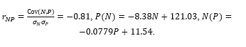
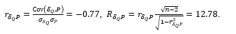
In fact, if one denotes the horizontal and vertical directions in Table 6 by and , respectively, one can obtain the corresponding sample means (i.e., , ) and dispersions (i.e., , ), as well as the mean-square deviations (i.e., , ) and the covariance (i.e., ). The later three values give one the correlation coefficient between the number of the tortuosity arcs and the relative blood flow rate loss in the investigated tortuous coronary arteries, viz.

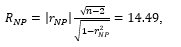
Further comparison of the coefficient significance,

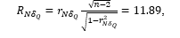
with the corresponding critical value, , (found from the Student’s table with the significance level and the degree of freedom , as well as the number of explaining variables , and the total number of the selected patients, ) allows one to conclude about statistical significance of the coefficient (i.e., ). This indicates strong correlation between the tortuosity severity12 and the relative blood flow rate loss in the tortuosity.

As for the magnitudes and , they can be found from the corresponding regression lines’ equations. In fact, based on the above data, the equations for the regression lines and can be written as

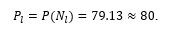
Then substituting the above critical value into the later equation yields

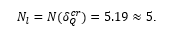
This indicates that a tortuosity with at least 5 arcs should be hemodynamically significant. This agrees reasonably well with the corresponding conclusion made in analyzing Table 4.

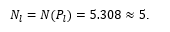
The obtained value of allows one to determine from the first of the above two equations, viz.

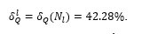
One can see that the obtained value of correlates well with the corresponding critical one, .

The next two tables show one the correlation between the number of the tortuosity arcs, , and the rate of angina pectoris attacks, , calculated in points (Table 7), as well as that between and the relative blood flow rate loss, , (Table 8) in the selected patients. If one denotes the horizontal and vertical directions in Table 7 by and , respectively, and determines the corresponding sample means and dispersions for the data of the table (i.e., , , , ), then one can see that the corresponding mean-square deviations, and , and the covariance, , have the following values

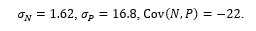
These magnitudes yield the correlation coefficient between and for the investigated tortuous coronary arteries, , as well as equations for the corresponding regression lines, and , viz.

Table 7: Distribution of the patients with SCAT of the AIVB of the LCA vs and .

, points	, %						Total, n
	20-30	30-40	40-50	50-60	60-70	70-80
0-9							0
10-19						1	1
20-29					1		1
30-39				2	1	2	5
40-49			1	3	2		6
50-59			3	7	3	1	14
60-69			8	14	3		25
70-79		3	9	14	1		27
80-89	1	16	3	1			21
90-99	5	7					12
Total, n	6	26	24	41	11	4	112

Table 8: Distribution of the patients with SCAT of the AIVB of the LCA vs and .

Further comparison of the coefficient significance,

with the corresponding critical value given above, , indicates statistical significance of the coefficient (i.e., )., and hence, strong correlation between the tortuosity severity12 and the rate of angina pectoris attacks.

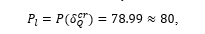
In its turn, the above equation allows one to determine approximately the critical value for the rate of angina pectoris attacks, , starting from which the corresponding tortuosity can be expected to be hemodynamically significant, viz.

On the other hand, the obtained magnitude yields, on the basis of the regression line equation , the corresponding value for , viz.

This correlates reasonably well with the above two predictions for made on the basis of the method.

Similar analysis of Table 8 (whose horizontal and vertical directions are denoted by and , respectively) allows one to conclude about strong correlation between the relative blood flow rate loss in the considered tortuous coronary arteries and the rate of angina pectoris attacks in the corresponding patients. Indeed, for the data of Table 8, the corresponding sample means and dispersions are , and , , respectively. They give one the corresponding mean-square deviations, and , as well as the covariance, . From these values one obtains the correlation coefficient between and together with its significance, viz.

Then the comparison of the obtained magnitude with confirms strong correlation between and .

Then the comparison of the obtained magnitude with confirms strong correlation between and .

In addition to these, the indicated statistical characteristics of Table 8 allow one to find the corresponding regression lines’ equations, viz.

The first of them gives one the value of , viz.

which correlates well with the corresponding one determined from Table 7.

In its turn, the obtained value of allows one to determine from the second regression line equation, viz.

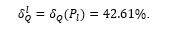
This magnitude agrees well with the corresponding one found from Table 6.

Finally, the data of the last two tables allow one to conclude about strong correlation between the number of the tortuosity arcs, , and the functional class of patients, FC, (Table 9), as well as about that between the relative blood flow rate loss, , and the functional class (Table 10) in the selected 112 patients. In fact, the statistical characteristics of interest for these tables are as follows

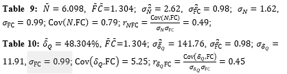
(here the horizontal and vertical directions in Table 9 are denoted by and FC, whereas in Table 10 by and FC). From this one can see that the significance of the correlation coefficient for each table,

exceeds the corresponding critical value, . This confirms the above conclusion about strong correlation between and FC, as well as about that between and FC.

FC								Total, n
	3	4	5	6	7	8	9
0	3	10	7	3	2	1	1	27
1	1	4	7	10	10	4	2	38
2		4	7	9	7	6	2	35
3				1	2	4	3	10
4						1	1	2
Total, n	4	18	21	23	21	16	9	112

Table 9: Distribution of the patients with SCAT of the AIVB of the LCA vs and FC.

FC	, %						Total, n
	20-30	30-40	40-50	50-60	60-70	70-80
0	1	13	8	2	3		27
1	4	9	8	15	1	1	38
2	1	4	6	18	5	1	35
3			2	6	2		10
4						2	2
Total, n	6	26	24	41	11	4	112

Table 10: Distribution of the patients with SCAT of the AIVB of the LCA vs and FC.

1. An approximate method has been developed to allow cardiologists to find (with satisfactory precision and speed) both quantitative changes in the blood flow characteristics of interest in larger coronary arteries, caused by the appearance of their pathological tortuosity, and a hemodynamic significance of those changes based on the data taken from the appropriate coronarographies only.
2. This method is based on replacement of real blood flows in the originally healthy and subsequently pathologically tortuous coronary artery with the corresponding cross-sectionally averaged ones, subsequent obtaining the blood flow characteristics of interest in terms of the corresponding averaged flow characteristics and making a comparative analysis of the appropriate obtained flow characteristics with one another.
3. The method allows one not to take account of a number of identical factors for the originally healthy and subsequently pathologically tortuous segment of the coronary artery under investigation (such as arterial pressure, the number of heartbeats, the inflow rate in the segment, mass density, viscosity and temperature of the blood, the physical and geometrical characteristics of the arterial wall, etc.). In addition, it gives one the possibility to determine the blood flow characteristics of concern at any time after carrying out a coronarography, is not associated with solving complicated technical problems, and does not require special facility to be used, special professional training and significant temporal and financial expenses.
4. Based on the analysis of coronarographies of 112 patients with SCAT of the AIVB of the LCA and the method developed, it was found that 80 patients (i.e., 71.4%) had hemodynamically significant tortuosity. Herewith the time, needed to decide on each patient immediately after making the coronarography, did not exceed 2 hours.
5. It was found that the hemodynamic significance of the tortuosity generally increases/decreases as the number of the tortuosity arcs increases/decreases. However, there were cases when tortuosities with the bigger number of arcs were hemodynamically less significant compared to those having the smaller number of arcs. It can be explained by the corresponding dependence of hemodynamic resistance of the tortuosity on the heights and the widths of the tortuosity arcs, their ratios, etc. However, obtaining a functional dependence of the resistance on the noted parameters requires carrying out extensive appropriate investigations.
6. Based on the method, a strong correlation between (i) the tortuosity severity12 and the corresponding relative blood flow rate loss, (ii) the tortuosity severity and the rate of the corresponding angina pectoris attacks, (iii) the relative blood flow rate loss and the rate of the corresponding angina pectoris attacks, (iv) the tortuosity severity and the functional class of the corresponding patients, (v) the relative blood flow rate loss and the functional class of the corresponding patients was found for the considered tortuosities. This suggests a strong independent influence of the coronary artery tortuosity on the clinical symptoms of patients with ischemic heart disease, cardiac syndrome X and severe coronary artery tortuosity.
7. The critical values for the number of the tortuosity arcs, the relative blood flow rate loss and the rate of angina pectoris attacks were obtained, starting from which the corresponding tortuosity can be hemodynamically significant.
8. The results obtained within the framework of the method and their analysis made create a good background for future application of the method in clinical practice.

The author expresses gratitude to the Chief Doctor of the Saint Catherine’s cardiological clinic (Odessa, Ukraine) Dr. D. M. Sebov for his stimulation of and promotion to making the research described in this paper, as well as for the corresponding materials provided and the useful comments given by him in discussing this work. Thanks, are also expressed to all personnel of the clinic who directly or indirectly helped to carry out this research. A major part of the financial expenses related to the research was covered by the clinic.